1. Talking to Computers: Turning Ideas into Instructions

1.1. Learning Objectives

By the end of this chapter, you will be able to:

1. Set up and use the course computing environment (JupyterLab and basic command-line navigation).

2. Write and run simple Python code using variables, basic types, and print statements.

3. Control program flow with correct indentation using if/elif/else.

4. Use loops to automate repetition with for and while.

5. Define and use functions to package reusable computations.

6. Work with basic data structures (lists and dictionaries) for storing and accessing data.

7. Use Git at a basic level to obtain the course repository and manage simple updates/changes safely.

Note (KSU students): See Appendix A: KSU Infrastructure (Timur / VPN / JupyterHub) for KSU-specific setup.

1.2. Introduction

1.2.1. Machine Language

Computers always do exactly as they are told! Instructions they understand are in a machine language.

But when writing and running programs, we communicate to the computer through “shells”, in high-level languages (e.g. Python, Java, Fortran, C, …), or through problem-solving environments (e.g. Maple, Mathematica, Matlab, …).

Eventually these commands/programs are translated into the basic machine language that the hardware understands.

1.2.2. Shells, Operating Systems and Compilers

A shell is a command-line interpreter: a small set of programs run by a computer that respond to the commands that you key in. The job of the shell is to run programs, compilers and utilities. A demonstration of this will be given during the lectures, but we won’t be using shells extensively. See the next section for more details!

Operating systems, e.g. Unix, DOS, Linux, MacOS, Windows, are a group of programs used by the computer to communicate with users and devices, to store and read data, and to execute programs.

When you submit a program to your computer in a high-level language, the computer uses a compiler to process it. The compiler translates your program into machine language.

Fortran and C (e.g.) read the entire program and then translate it into basic machine instructions. These are known as “compiled languages”.

BASIC/Maple translate each line of program as it is entered. These are “interpreted languages”.

Python and Java are a mix of both.

1.2.3. Files and Folders

In analogy to physical filing cabinets containing folders which in turn contain files, computers store information in files that reside in folders, or “directories”. Folders can also contain other folders, or a mixture of files and folders, and so on.

1.2.4. The Unix Terminal (or Shell)

A terminal is a text-based interface that allows users to interact directly with a Unix-like operating system (such as Linux or macOS) by typing commands.

If you have a macOS or Linux computer, then you should already have a terminal application installed. On the MacOS, it’s just called “Terminal”.

On Windows, I recommend installing the Ubuntu distribution through the “Windows Subsystem for Linux” (see https://learn.microsoft.com/en-us/windows/wsl/install).

Some basic terminal commands are:

command	result
ls	Lists directory contents.
cd	Changes the current directory.
pwd	Prints the current working directory.
mkdir	Creates a new directory.
touch	Creates a new file or updates the timestamp of an existing file.
rm	Removes files or directories.
cp	Copies files or directories.
mv	Moves files or directories.
cat	Concatenates and displays the content of files.
grep	Searches for patterns in files.
man	Displays the manual pages of commands.
clear	Clears the terminal screen.

1.2.5. Appendix A: KSU Infrastructure (Timur / VPN / JupyterHub)

Note

KSU-only setup details go here. Non-KSU students can ignore this section.

This section contains specifics on how to connect to Kennesaw State University’s Timur workstation, and can be safely ignored if you are not actually attending the course!

Remote Connection via SSH

To connect to a remote computer, we use the “Secure Shell Protocol” (ssh), a cryptographic network protocol for operating network services securely over an unsecured network.

To access KSU’s Timur:

Using your terminal type:

ssh -Y username@timur.kennesaw.edu

where username is your given username.

Then enter your password. If this is your first time, change your password by typing:

passwd

Note that sometimes you may not see a response when typing in a password in the terminal!

Type

exit to disconnect.

Logging into the JupyterHub Server

1. If you are not on the KSU network while at KSU, you will first need to use the GlobalProtect VPN. If you are at KSU and still can’t connect (e.g. you get ```ssh: Could not resolve hostname blah.blah: nodename nor servname provided, or not known’’’) then try connecting to the VPN.

2. Open a Terminal locally (meaning, on your computer, and not while ssh’d into timur!) and create a secure forwarding port by typing:

ssh -N -f -L 8887:localhost:8000 username@timur.kennesaw.edu

where username is your username. You will be asked to enter your password.

Notes:

• The password will be hidden, so don’t expect any feedback when typing the password!

• If you get an error related to the port 8887, try another port, such as 8888 or 7777.

• On Windows, it seems like there is no response after entering the password. Simply keep the terminal open and go to the next step.

3. then navigate with your web browser to:

localhost:8887,

(or the appropriate port you attached the remote server to as above).

This will ask you again for your username and password. If you encounter an error once you reach the page, simply click on the banner (upper left) and start the server again.

4. Open up a JupyterLab file by double-clicking it. This should load the default kernel, which does not have all the packages installed. To make sure you are using the right kernel, click on the upper-right corner, and choose “Python (CompPhys)”.

It is recommended that you create new files to write and test code.

1.2.6. Structure and Reproducible Program Design

Programming is a written art that blends the elements of science, math, and computer science into a set of instructions that permit a computer to accomplish a desired task.

It is important that the source code of your program itself is available to others so that they can reproduce and extend your results.

Reproducibility is an essential ingredient in science.

In addition to the grammar of the computer language, a scientific program should include a number of essential elements to ensure the program’s validity and usability.

As with other arts, it is recommended that until you know better, you should follow some simple rules:

A good program should:

• give correct answers.

• be clear and easy to read, with the action of each part easy to analyze.

• document itself for the readers/programmer.

• be easy to use.

• be built out of small programs that can be independently verified.

• be easy to modify and robust enough to keep giving correct answers after modification and simple debugging.

• document the data formats used.

• use trusted libraries.

• be published or passed onto others to use and to develop further.

An elementary way to make any program clear is to structure it with indentation, skipped lines, parentheses, all placed strategically.

Python uses indentation as a structure element, as well as for clarity. We will discuss indentation below.

1.2.7. Git and Version Control

We will make use of git, a version control system to keep track of changes to the course repository. I also recommend that you use git for your own projects. For a full description of git, see the free Pro Git book: https://git-scm.com/book/en/v2.

Version control records changes to a file or set of files over time so that you can go back to specific versions later. Typically, there exists a single server (a server = a computer whose job is to provide a service that other devices ask for) that contains all the files of your project, also known as a repository, that you wish to “commit” changes to. The advantage of git and other distributed version control systems is that you can keep a local copy of the repository, including the full history.

There are several commercial platforms that can host your projects. One example is GitHub (github), which we will be using in this course. This book, and its corresponding repository, is hosted there.

See https://git-scm.com/book/en/v2/Getting-Started-Installing-Git for how to get git installed on your system. Timur already has a git installation.

If you wish to obtain a copy of an existing repository, you need to clone it. For this course:

git clone https://github.com/apapaefs/ScientificComputing.git

This will create the ScientificComputing/ directory on your filesystem, reflecting all the files of the repository.

You can also create your own local repository (e.g., on Timur) as follows:

mkdir my_project
cd my_project
git init

The first line creates a new directory called my_project, then the second line changes your location into that directory, and the third line creates the repository. At this point nothing in your project is being tracked yet.

Let’s say you have created a JupyterLab notebook in the my_project/ directory called My_Project.ipynb and you want to track changes. Then you need to add it to the repository:

git add My_Project.ipynb
git commit -m "Initial project version"

If you wish to check which files have been changed in your local repository, you can use:

git status

You can commit changes to My_Project.ipynb at any time, e.g.:

git commit -m "Minor change to code"

If you have changes that you don’t want to keep, you can restore the file to what it looked like when you last committed:

git restore My_Project.ipynb

You can also use git to collaborate on a project through remote repositories (such as on GitHub).

While working with the course repository, you will inevitably change files (e.g., when running or modifying the JupyterLab notebooks). I recommend you create copies of notebooks while you are working with them.

Tip

Safe workflow for the course repository

You will inevitably modify notebooks while working. Best practice: make a personal copy and work on that copy.

Example:

• Duplicate SomeNotebook.ipynb → SomeNotebook_MyWork.ipynb

• Or create a MyWork/ folder and keep your copies there

Updating the course repo (safe first)

Run these inside the ScientificComputing/ directory:

git status
git pull

If git pull complains because you have local changes, do not use reset --hard yet. Use one of the safe options below.

Undoing changes (safe options)

Option A: Discard changes in a single file (uncommitted):

git restore path/to/file.ipynb

Option B: Discard all uncommitted changes (tracked files):

git restore .

Option C: Save your changes temporarily, then update:

git stash -u
git pull
git stash pop

Last resort: restore the repository exactly to the remote version (DESTRUCTIVE)

This will overwrite local work and delete untracked files.

Before doing this, make a backup copy of any notebook you care about.

git fetch origin
git checkout main
git reset --hard origin/main
git clean -fd

1.3. A Brief Introduction to Python

From the Python tutorial: https://docs.python.org/3/tutorial/index.html

“Python is an easy to learn, powerful programming language.

It has efficient high-level data structures and a simple but effective approach to object-oriented programming.

Python’s elegant syntax and dynamic typing, together with its interpreted nature, make it an ideal language for scripting and rapid application development in many areas on most platforms.”

Today we will learn how to use Python in a JupyterLab notebook (such as this one) and use it to solve some basic problems, including visualization.

1.3.1. What is Python?

Python is an interpreted, interactive, object-oriented programming language. It incorporates modules, exceptions, dynamic typing, very high level dynamic data types, and classes.

1.3.2. Aside: Why is it called that?!

When he began implementing Python, Guido van Rossum was also reading the published scripts from “Monty Python’s Flying Circus”, a BBC comedy series from the 1970s. Van Rossum thought he needed a name that was short, unique, and slightly mysterious, so he decided to call the language Python.

1.3.3. JupyterLab Notebooks and First Code

There are many ways to use Python. It can be used directly in a shell (terminal), but I will mainly be using JupyterLab notebooks, such as the one you are currently looking at.

JupyterLab is a web-based, interactive development environment for notebooks, code, and data. Here, we will use it to run Python code.

First, log into the JupyterHub server on Timur as described above.

After you have performed step 4, you should have a new notebook open called Untitled.ipynb. You can write code in there.

As a first test, let’s load the NumPy (numerical Python) module and use it to get the value of π. We will discuss modules later in this chapter.

Type:

import numpy as np

print("The value of pi is", np.pi)

The first line imports the NumPy module, giving it the name np. The second line prints the text that you see between the quotation marks “” and then the value of np.pi, which corresponds to π.

The print command takes as input strings separated by commas. In this case the first string is "The value of pi is" and the second string is the decimal number np.pi, converted into a string.

To “execute” the block of code, make sure it is currently active and either press the “play” button on the JupyterLab panel, or hit Shift-Enter.

If this successful, then congratulations, you’ve written your first Python script!

You can also use Python to calculate the value of \(π^2\). In the same notebook, add in a following block:

pisq = np.pi**2 

This has created a new variable called pisq and assigned it to the value of \(π^2\). In Python, a**b means \(a^b\).

You can now print it by adding:

# The next line will print the value of $π^2$, along with some text 
print("The value of pi^2 is", pisq)

Note that JupyterLab notebooks in general, automatically print the output of the last line of code in a cell, provided that line is an expression or variable that evaluates to a value.

Anything that starts with # will not be read by Python. These are comments. Comments are a very important part of the code. They can provide notes on the structure of the code, caveats, warnings, things to be aware of, potential pitfalls, all for the purpose that a human (including the future you!) will be able to understand what the program is supposed to be doing. We will be discussing how to construct good comments for your code in the duration of the course. For a more advanced view, see https://stackoverflow.blog/2021/12/23/best-practices-for-writing-code-comments/.

Warmup Exercise: Figure out how to get the value of the Euler constant from NumPy! (See the NumPy manual on the web).

1.3.4. Debugging Quickstart: Reading Errors and Fixing Them

When you run code, errors are normal. Debugging is the process of reading what the computer tells you, making a small change, and trying again. In this course, you will see most errors in JupyterLab as a traceback (a stack of lines ending with an error type and message).

Tip

A reliable way to read a traceback (do this every time)

1. Read the last line first. It contains the error type (e.g., NameError) and a short message.

2. Find the first line that points to your code. In a notebook, it will reference the cell you ran.

3. Identify the exact “trigger.” A variable name, a missing :, mismatched parentheses, wrong indentation, etc.

4. Make one small change. Then run the cell again.

5. If results feel inconsistent: use Kernel → Restart Kernel and Run All to reset the state and run cells in order.

Common JupyterLab-specific gotchas

• Execution order matters. If you define a variable in a cell but never ran that cell, the variable does not exist.

• Restarting the kernel clears memory. After a restart, you must re-run cells that define variables/functions before using them again.

Common errors and the first thing to try

• NameError: You used a name that does not exist (misspelling, not defined yet, or you did not run the defining cell).

• SyntaxError: Python cannot parse the code (missing :, mismatched quotes/parentheses, invalid characters).

• IndentationError: The indentation does not form a valid block (misaligned code, mixing tabs/spaces, missing indent after :).

• TypeError: You applied an operation to the wrong type (e.g., adding a string and an integer).

• ModuleNotFoundError: The package is not installed in the current environment, or you are using the wrong kernel.

• IndexError / KeyError: You tried to access a list index that does not exist, or a dictionary key that is not present.

1.3.5. Variables in Python

Variables in code are symbolic names that are stored on the computer’s memory. You can think of them in the same way as in a math problem, where e.g. you say \(x = 3\).

In Python you can define variables of any type using the = sign, e.g.:

NumberOfEggs = 3
String1 = "Break the"
String2 = "eggs"

In the first line, we defined NumberOfEggs as an integer, and in the second and third lines as strings.

Note that in Python, as opposed to e.g. C++, you do not need to specify the type of variable. It is automatically determined by the value that you assign it to. Python is said to be a “dynamically typed” language.

1.3.6. Python as a Calculator

We already saw how to calculate squares of numbers in Python. In fact, you can use Python as a fully-fledged calculator, e.g.:

2 + 3

5

2 * 42

84

8/5

1.6

Note that the above is a float of double precision! (see later)

3**2

9

And you can use variables during these operations:

NumberOfEggs * 2

6

1.3.7. Manipulating Strings

It’s very easy to manipulate text in Python (i.e. strings). You can define strings as above, and you can use either double or single quotation marks: “” or ‘’.

Let’s create a new string from the three available strings:

String3 = String1 + " " + str(NumberOfEggs) +  " " + String2
print(String3)

Break the 3 eggs

Strings can be indexed, e.g. you can access the a certain “letter” in a string by using a number enclosed by []. Note that in Python, numbering starts at 0. This does not apply to all programming languages!

Let’s access the first letter in the newly-created String3:

String3[0]

'B'

or the second letter:

String3[1]

'r'

You can use negative integers to start counting from the right. E.g. the last letter in the string can be accessed via:

String3[-1]

's'

and then you can continue “moving” to the right by “going more negative”, e.g. the penultimate letter in the string can be accessed by:

String3[-2]

'g'

You can also “slice” strings to obtain a portion of them. E.g. for the first 2 letters”

String3[0:2]  # characters from position 0 (included) to 2 (excluded)

'Br'

or the 3rd to 5th letter:

String3[2:5]  # characters from position 2 (included) to 5 (excluded)

'eak'

or the 5th letter to the end:

String3[4:]   # characters from position 4 (included) to the end

'k the 3 eggs'

len() tells you how long a string is:

len(String3)

16

So the valid “positions” within the string would be 0 (first element) to 15 (last element).

1.3.8. Lists in Python

Lists are used to group together values. They are written as a list of comma-separated values (items) between square brackets. They may contain items of different types but usually the items all have the same type.

For example, the list containing the squares of the first 5 integers is given by:

squares = [1, 4, 9, 16, 25]

Like strings, lists can be indexed and sliced:

squares[3]  # indexing returns the item

16

squares[-1] # indexing returns the last item

25

squares[1:] # returns the second element up to the end

[4, 9, 16, 25]

Lists also support operations like concatenation:

squares + [36, 49, 64, 81, 100]

[1, 4, 9, 16, 25, 36, 49, 64, 81, 100]

Unlike strings, which are immutable, lists are a mutable type, i.e. it is possible to change their content:

cubes = [1, 8, 27, 65, 125]  # something's wrong here
4 ** 3  # the cube of 4 is 64, not 65!

64

cubes[3] = 64  # replace the wrong value
cubes

[1, 8, 27, 64, 125]

You can also add new items at the end of the list, by using the list.append() method:

cubes.append(216)  # add the cube of 6
cubes.append(7 ** 3)  # and the cube of 7
cubes

[1, 8, 27, 64, 125, 216, 343]

len() also applies to lists:

len(cubes)

7

len(cubes)

7

1.4. Control Flow Tools

1.4.1. if Statements and Python Indentation

One of the most well-known statement type is the if statement. An example:

# Choose a value for the integer x:
x = 10 # NOTE: a single equal sign ASSIGNS a value to x! 
# Then check various cases with an if ... elif ... else statement:
if x < 0: 
    x = 0
    print('Negative integer detected, changed to zero!')
elif x == 0: # NOTE: a double equal sign CHECKS the value! 
    print("Zero")
elif x == 1:
    print("One")
else: 
    print("Positive integer, not one")

Positive integer, not one

‘elif’ is short for ‘else if’, there can be any number of such statements (including none). ‘else’ is optional and is ‘triggered’ if all other statements are not satisfied.

It’s important to note that a single equal sign, e.g. x=10, assigns a value, whereas the double equal sign == checks the equality. This is a common mistake when programming so be sure to remember to use the correct symbols.

To check values, you can also use the standard mathematical symbols <, > and for greater/less than or equal you can use >= and <= respectively.

For the first time in the above code we also see the importance of indentation in Python. It’s very important to indent correctly to obtain the desired result. Consider the following example of an if statement:

age = 18.5

if age >= 18:
    print("You can vote.")   # inside the if-block (runs only if condition is true)

print("Done.")               # outside the if-block (runs no matter what)

You can vote.
Done.

The first print statement is executed inside the if statement and the second outside it.

Now consider the nested statement, that first checks your age for an event that requires you to be over 18 and then whether you have a ticket for the event:

age = 21
has_ticket = False

if age >= 18:
    print("Over 18! You may enter the event.")
    if not has_ticket:
        print("But you need a ticket to get in.")
    else:
        print("Ticket verified. Welcome!")
print("Done.")

Over 18! You may enter the event.
But you need a ticket to get in.
Done.

The second if statement will only be considered if the first one is true!

We have also introduced the value False or True, for a variable in Python above.

But now let’s see what happens when you don’t indent properly:

age = 17
has_ticket = False

if age >= 18:
    print("Over 18! You may enter the event.")
if not has_ticket:
    print("But you need a ticket to get in.")
else:
    print("Ticket verified. Welcome!")
print("Done.")

But you need a ticket to get in.
Done.

The age is checked independently of whether you have a ticket for the event, and we get a redundant printout (since you wouldn’t be able to enter regardless of whether you have a ticket or not, since you are underage).

To conclude: make sure you indent properly in Python!

1.4.2. for and while Statements

Python’s for statement iterates over the items of any sequence (e.g. a list or a string), in the order they appear in the sequence. In the example below, w becomes each word in the words list every time you “loop” through:

# measure the length of all the strings in a list:
words = ['Einstein', 'Galileo', 'Copernicus']
for w in words: 
    print(w, len(w)) # print w and the length of w in each iteration

Einstein 8
Galileo 7
Copernicus 10

If instead you want to iterate over the sequence of numbers, the range() function comes in handy:

for i in range(3):
    print(words[i], len(words[i])) 

Einstein 8
Galileo 7
Copernicus 10

or, equivalently:

for i in range(len(words)):
    print(i, words[i], len(words[i]))

0 Einstein 8
1 Galileo 7
2 Copernicus 10

A while statement continues until the given condition stops being true:

j = 0
while j < 3:
    print(j, words[j], len(words[j]))
    j = j + 1 # this line is ESSENTIAL: otherwise you end up with an INFINITE loop!

0 Einstein 8
1 Galileo 7
2 Copernicus 10

Let’s use a while loop to write down the first few terms in the Fibonacci series:

# Fibonacci series:
# the sum of two elements defines the next
a = 0
b = 1 # define the first two
while a < 10: # do this while the number a is less than 10, stop when it exceeds 10.
    print(a) # print the next number in the series
    c = b
    b = a+c # a becomes the next number to be printed, and calculate the one after that.
    a = c

0
1
1
2
3
5
8

1.4.3. break and continue Statements, and else Clauses on Loops

The break statement breaks out the innermost enclosing for or while loop. E.g.:

for w in words:
    if w == 'Galileo': 
        break # once Galileo is found, break the loop!
    print(w)

Einstein

The continue statement skips the rest of the loop, e.g.:

for w in words:
    if w == 'Galileo': 
        continue # once Galileo is found, skip the rest of the loop (don't print in this case)
    print(w)

Einstein
Copernicus

A for or while loop can include an else clause. In a for loop the else clause is executed after the loop reaches its final iteration. In a while loop, it’s executed after the loop’s condition becomes false. In either kind of loop, the else clause is not executed if the loop was terminated by a break.

In the following example, an else clause is used at the end of a for loop which contains an if statement that checks whether a number is divisible by all numbers smaller than itself. (The n % x part calculates the remainder of the division n/x).

for n in range(2,10):
    for x in range(2, n):
        if n%x==0:
            print(n, 'equals', x, '*', n/x)
            break # we have found a number smaller than n is a factor of n, so n is not a prime number! -> break the for loop here -> else is not executed!
    else: 
        # loop fell through without finding a factor 
        print(n, 'is a prime number')

2 is a prime number
3 is a prime number
4 equals 2 * 2.0
5 is a prime number
6 equals 2 * 3.0
7 is a prime number
8 equals 2 * 4.0
9 equals 3 * 3.0

The continue statement continues with the next iteration of the loop:

for num in range(2, 10):
    if num % 2 == 0:
        print("Found an even number", num)
        continue
    print("Found an odd number", num)

Found an even number 2
Found an odd number 3
Found an even number 4
Found an odd number 5
Found an even number 6
Found an odd number 7
Found an even number 8
Found an odd number 9

Warmup Exercises with for and while loops:

Exercise 1:

Predict the output of the following loop:

for i in range(5):
    print("i is", i)
print("Done")

Exercise 2:

Write code that prints this pattern exactly:

*
**
***
****
*****

Exercise 3:

We want to write code that performs a countdown to zero from a certain number. A student wrote some code that looks like this:

count = 5

while count > 0:
    print(count)

print("Blastoff!")

What’s wrong with this code? Fix it so that the it counts down to zero and stops!

Exercise 4:

You have a list of item prices. Everyone pays the sum. Only members get a 10% discount, and only on items over $20. Using the code below, write a function that calculates how much a customer will pay:

prices = [12, 25, 8, 40]
is_member = True

total = 0

for price in prices:
    total += price
    # TODO: Apply a 10% discount ONLY if:
    # 1) is_member is True, AND
    # 2) price > 20
    # (Discount means subtract 10% of that price from total.)

print("Final total:", total)

1.5. Defining Functions

In Python, a function is like a mathematical function: you give it an input (arguments), it applies a defined set of steps, and it returns an output (a result), so you can reuse the same “rule” whenever you need it. For example, let’s say you have the function \(x sin(x)\) and you want to avoid typing this over and over again:

import numpy as np
def f(x):
    return x * np.sin(x)

The keyword def introduces a function definition. It must be followed by the function name and the parenthesized list of formal parameters. The statements that form the body of the function start at the next line, and must be indented. The first statement of the function body can optionally be a string literal; this string literal is the function’s documentation string.

We can execute the function by calling it with a parameter, e.g.:

f(np.pi/2) # we expect this to be π/2 * sin(π/2) = π/2:

np.float64(1.5707963267948966)

We can create a function that writes the Fibonacci series to an arbitrary boundary:

def fib(n):    # write Fibonacci series up to n
    """Print a Fibonacci series up to n."""
    a, b = 0, 1
    while a < n:
        print(a, end=' ')
        a, b = b, a+b

Let’s execute the function to calculate the Fiobonacci series up to n:

fib(2000)

0 1 1 2 3 5 8 13 21 34 55 89 144 233 377 610 987 1597 

Functions without return statements return None

fib(2000)

0 1 1 2 3 5 8 13 21 34 55 89 144 233 377 610 987 1597 

We can instead create a function that returns the values we are after, e.g. in a list:

def fib2(n):  # return Fibonacci series up to n
    """Return a list containing the Fibonacci series up to n."""
    result = []
    a, b = 0, 1
    while a < n:
        result.append(a)    # see below
        a, b = b, a+b
    return result

And we can call it to create a list, e.g. fib100:

f100 = fib2(100)

print(f100)

[0, 1, 1, 2, 3, 5, 8, 13, 21, 34, 55, 89]

Note that append is a method that acts on the list object result to add a new element at its end.

For more details on defining functions, see https://docs.python.org/3/tutorial/controlflow.html#more-on-defining-functions. We will discuss some of those aspects where necessary during the course.

1.6. Data Structures

1.6.1. Further Details on Lists

We already mentionewd the list.append() method for a list. The list data type has some more methods, some of which are:

• list.append(x): Add an item to the end of the list. Equivalent to a[len(a):] = [x].

• list.insert(i, x): Insert an item at a given position. The first argument is the index of the element before which to insert, so a.insert(0, x) inserts at the front of the list, and a.insert(len(a), x) is equivalent to a.append(x).

• list.remove(x): Remove the first item from the list whose value is equal to x. It raises a ValueError if there is no such item.

• list.pop([i]): Remove the item at the given position in the list, and return it. If no index is specified, a.pop() removes and returns the last item in the list. (The square brackets around the i in the method signature denote that the parameter is optional, not that you should type square brackets at that position. You will see this notation frequently in the Python Library Reference.)

• list.clear(): Remove all items from the list.

• list.count(x): Return the number of times x appears in the list.

• list.reverse(): Reverse the elements of the list in place.

• list.sort(*, key=None, reverse=False): Sort the items of the list in place (the arguments can be used for sort customization, see sorted() for their explanation).

• list.reverse(): Reverse the elements of the list in place.

• list.copy(): Return a shallow copy of the list. Equivalent to a[:].

The following examples use several of the list methods:

fruits = ['orange', 'apple', 'pear', 'banana', 'kiwi', 'apple', 'banana']

fruits.count('apple')

2

fruits.count('tangerine')

0

fruits.index('banana')

3

fruits.index('banana', 4)  # Find next banana starting at position 4

6

fruits.reverse()
fruits

['banana', 'apple', 'kiwi', 'banana', 'pear', 'apple', 'orange']

fruits.append('grape')
fruits

['banana', 'apple', 'kiwi', 'banana', 'pear', 'apple', 'orange', 'grape']

fruits.sort()
fruits

['apple', 'apple', 'banana', 'banana', 'grape', 'kiwi', 'orange', 'pear']

fruits.pop()

'pear'

1.6.2. List Comprehensions

List comprehensions provide a concise way to create lists. Common applications are to make new lists where each element is the result of some operations applied to each member of another sequence or iterable, or to create a subsequence of those elements that satisfy a certain condition.

E.g. let’s assume we want to create a list of squares, like:

squares = []
for x in range(10):
    squares.append(x**2)
squares

[0, 1, 4, 9, 16, 25, 36, 49, 64, 81]

We can instead use a list comprehension:

squares = [x**2 for x in range(10)]
squares

[0, 1, 4, 9, 16, 25, 36, 49, 64, 81]

A list comprehension consists of brackets containing an expression followed by a for clause, then zero or more for or if clauses. The result will be a new list resulting from evaluating the expression in the context of the for and if clauses which follow it.

E.g. Let’s say we want the even numbers in the squares list:

even_squares = [y for y in squares if y%2 == 0]
even_squares

[0, 4, 16, 36, 64]

1.6.3. Tuples and Sequences

We saw that lists and strings have many common properties, such as indexing and slicing operations. They are two examples of sequence data types (see Sequence Types — list, tuple, range). There is also another standard sequence data type: the tuple.

A tuple consists of a number of values separated by commas, for instance:

t = 12345, 54321, 'hello!'
t[0]

12345

# Tuples may be nested:
u = t, (1, 2, 3, 4, 5)
u

((12345, 54321, 'hello!'), (1, 2, 3, 4, 5))

As you see, on output tuples are always enclosed in parentheses, so that nested tuples are interpreted correctly; they may be input with or without surrounding parentheses, although often parentheses are necessary anyway (if the tuple is part of a larger expression). It is not possible to assign to the individual items of a tuple, however it is possible to create tuples which contain mutable objects, such as lists.

Though tuples may seem similar to lists, they are often used in different situations and for different purposes. Tuples are immutable, and usually contain a heterogeneous sequence of elements that are accessed via unpacking (see later) or indexing. Lists are mutable, and their elements are usually homogeneous and are accessed by iterating over the list.

# Tuples are immutable:
#t[0] = 88888
# Uncomment above line to execute and get an error!

1.6.4. Dictionaries

Another useful data type built into Python is the dictionary. Unlike sequences, which are indexed by a range of numbers, dictionaries are indexed by keys, which can be any immutable type; strings and numbers can always be keys. Tuples can be used as keys if they contain only strings, numbers, or tuples; if a tuple contains any mutable object either directly or indirectly, it cannot be used as a key. You can’t use lists as keys, since lists can be modified in place using index assignments, slice assignments, or methods like append() and extend().

It is best to think of a dictionary as a set of key: value pairs, with the requirement that the keys are unique (within one dictionary). A pair of braces creates an empty dictionary: {}. Placing a comma-separated list of key:value pairs within the braces adds initial key:value pairs to the dictionary; this is also the way dictionaries are written on output.

The main operations on a dictionary are storing a value with some key and extracting the value given the key. It is also possible to delete a key:value pair with del. If you store using a key that is already in use, the old value associated with that key is forgotten. It is an error to extract a value using a non-existent key.

Performing list(d) on a dictionary returns a list of all the keys used in the dictionary, in insertion order (if you want it sorted, just use sorted(d) instead). To check whether a single key is in the dictionary, use the in keyword.

Here is a small example using a dictionary:

tel = {'jack': 4098, 'sape': 4139}
tel['guido'] = 4127
tel

{'jack': 4098, 'sape': 4139, 'guido': 4127}

tel['jack']

4098

del tel['sape']
tel['irv'] = 4127
tel

{'jack': 4098, 'guido': 4127, 'irv': 4127}

list(tel)

['jack', 'guido', 'irv']

sorted(tel)

['guido', 'irv', 'jack']

'guido' in tel

True

'jack' not in tel

False

The dict() constructor builds dictionaries directly from sequences of key-value pairs:

dict([('sape', 4139), ('guido', 4127), ('jack', 4098)])

{'sape': 4139, 'guido': 4127, 'jack': 4098}

In addition, dict comprehensions can be used to create dictionaries from arbitrary key and value expressions:

{x: x**2 for x in (2, 4, 6)}

{2: 4, 4: 16, 6: 36}

When the keys are simple strings, it is sometimes easier to specify pairs using keyword arguments:

dict(sape=4139, guido=4127, jack=4098)

{'sape': 4139, 'guido': 4127, 'jack': 4098}

1.6.5. Looping Techniques

When looping through dictionaries, the key and corresponding value can be retrieved at the same time using the items() method:

knights = {'gallahad': 'the pure', 'robin': 'the brave'}
for k, v in knights.items():
    print(k, v)

gallahad the pure
robin the brave

When looping through a sequence, the position index and corresponding value can be retrieved at the same time using the enumerate() function.

for i, v in enumerate(['tic', 'tac', 'toe']):
    print(i, v)

0 tic
1 tac
2 toe

To loop over two or more sequences at the same time, the entries can be paired with the zip() function.

questions = ['name', 'quest', 'favorite color']
answers = ['lancelot', 'the holy grail', 'blue']
for q, a in zip(questions, answers):
    print('What is your {0}?  It is {1}.'.format(q, a))

What is your name?  It is lancelot.
What is your quest?  It is the holy grail.
What is your favorite color?  It is blue.

To loop over a sequence in sorted order, use the sorted() function which returns a new sorted list while leaving the source unaltered.

basket = ['apple', 'orange', 'apple', 'pear', 'orange', 'banana']
for i in sorted(basket):
    print(i)

apple
apple
banana
orange
orange
pear

Using set() on a sequence eliminates duplicate elements. The use of sorted() in combination with set() over a sequence is an idiomatic way to loop over unique elements of the sequence in sorted order.

basket = ['apple', 'orange', 'apple', 'pear', 'orange', 'banana']
for f in sorted(set(basket)):
    print(f)

apple
banana
orange
pear

1.7. Debugging Examples

Now that we have learned how to write a little bit of code, let’s look at examples of common errors and how to fix them.

1.7.1. NameError (variable not defined)

Run this in a cell:

print("The value is:", x)

You should see a NameError because x does not exist yet.

Fix it by defining x first:

x = 10
print("The value is:", x)

1.7.2. SyntaxError (Python grammar problem)

Run this cell:

age = 20

if age >= 18
    print("Over 18")

You should see a SyntaxError. In most cases, look for a missing : or mismatched parentheses/quotes.

Fix it:

age = 20

if age >= 18:
    print("Over 18")

Now add an else clause that prints “Under 18”.

1.7.3. IndentationError (block structure problem)

Run this cell:

age = 20

if age >= 18:
print("Over 18")

You should see an IndentationError because the print statement is not indented under the if.

Fix it:

age = 20

if age >= 18:
    print("Over 18")

Now change the indentation on purpose so that “Done” prints only when age >= 18:

1.7.4. TypeError (wrong type used in an operation)

Run this cell:

age = "20"
print(age + 1)

You should see a TypeError because “20” is a string, not a number.

There are two ways to fix this:

age = "20"
print(int(age) + 1)

or

age = 20
print(age+1)

### `IndexError` and `KeyError` (access problems)

Run this cell: 

```python
vals = [10, 20, 30]
print(vals[3])

You should see an IndexError because valid indices are 0, 1, 2.

Fix it by printing the last element:

vals = [10, 20, 30]
print(vals[-1])

Now run this:

person = {"name": "Ada", "age": 20}
print(person["major"])

Fix it by printing existing keys:

person = {"name": "Ada", "age": 20}
print(person["name"])
print(person["age"])

Tip

When something feels “mysteriously wrong”

If your output does not match what you expect and you are not sure why:

1. Save your work.

2. Use Kernel → Restart Kernel and Run All.

3. Re-run the cell that fails and read the traceback again from the last line upward.

This solves a large fraction of “stale state” issues in notebooks.

1.8. Modules

1.8.1. User-Defined Modules

If you quit from the Python interpreter and enter it again, the definitions you have made (functions and variables) are lost. The same happens when you open a new jupyter notebook. Therefore, if you want to write a somewhat longer program, you are better off using a text editor to prepare the input for the interpreter and running it with that file as input instead. This is known as creating a script. As your program gets longer, you may want to split it into several files for easier maintenance. You may also want to use a handy function that you’ve written in several programs without copying its definition into each program.

To support this, Python has a way to put definitions in a file and use them in a script or in an interactive instance of the interpreter. Such a file is called a module; definitions from a module can be imported into other modules or into the main module (the collection of variables that you have access to in a script executed at the top level and in calculator mode).

A module is a file containing Python definitions and statements. The file name is the module name with the suffix .py appended. Within a module, the module’s name (as a string) is available as the value of the global variable __name__. For instance, we have created a file called fibo.py in the current directory with the following contents:

# Fibonacci numbers module

def fib(n):    # write Fibonacci series up to n
    a, b = 0, 1
    while a < n:
        print(a, end=' ')
        a, b = b, a+b
    print()

def fib2(n):   # return Fibonacci series up to n
    result = []
    a, b = 0, 1
    while a < n:
        result.append(a)
        a, b = b, a+b
    return result

Let’s import this module:

import fibo

This does not add the names of the functions defined in fibo directly to the current namespace; it only adds the module name fibo there. Using the module name you can access the functions:

fibo.fib(1000)

0 1 1 2 3 5 8 13 21 34 55 89 144 233 377 610 987 

fibo.fib2(100)

[0, 1, 1, 2, 3, 5, 8, 13, 21, 34, 55, 89]

fibo.__name__

'fibo'

There is a variant of the import statement that imports names from a module directly into the importing module’s namespace. For example:

from fibo import fib, fib2
fib(500)

0 1 1 2 3 5 8 13 21 34 55 89 144 233 377 

There is even a variant to import all names that a module defines:

from fibo import *
fib(500)

0 1 1 2 3 5 8 13 21 34 55 89 144 233 377 

If the module name is followed by as, then the name following as is bound directly to the imported module. This is effectively importing the module in the same way that import fibo will do, with the only difference of it being available as fib.

import fibo as fib
fib.fib(500)

0 1 1 2 3 5 8 13 21 34 55 89 144 233 377 

It can also be used when utilising from with similar effects:

from fibo import fib as fibonacci
fibonacci(500)

0 1 1 2 3 5 8 13 21 34 55 89 144 233 377 

1.8.2. Standard Modules and the Standard Library

Python comes with a library of standard modules, described in a separate document, the Python Library Reference (“Library Reference” hereafter). The built-in function dir() is used to find out which names a module defines. It returns a sorted list of strings:

import fibo
dir(fibo)

['__builtins__',
 '__cached__',
 '__doc__',
 '__file__',
 '__loader__',
 '__name__',
 '__package__',
 '__spec__',
 'fib',
 'fib2']

For a longer introduction to the standard library, check out: https://docs.python.org/3/tutorial/stdlib.html. Here, we will go through a few basic modules, and we will introduce more during the course.

The math module gives access to the underlying C library functions for floating point math:

import math
math.cos(math.pi / 4)

0.7071067811865476

math.log(1024, 2)

10.0

The random module provides tools for making random selections:

import random
random.choice(['apple', 'pear', 'banana'])

'apple'

random.sample(range(100), 10)   # sampling without replacement

[58, 20, 14, 35, 96, 70, 41, 0, 17, 46]

random.random()    # random float

0.33059853143792306

random.randrange(6) 

4

The statistics module calculates basic statistical properties (the mean, median, variance, etc.) of numeric data:

import statistics
data = [2.75, 1.75, 1.25, 0.25, 0.5, 1.25, 3.5]
print(statistics.mean(data))
print(statistics.median(data))
print(statistics.variance(data))

1.6071428571428572
1.25
1.3720238095238095

1.8.3. NumPy

NumPy is the fundamental package for scientific computing in Python. It is a Python library that provides a multidimensional array object, various derived objects (such as masked arrays and matrices), and an assortment of routines for fast operations on arrays, including mathematical, logical, shape manipulation, sorting, selecting, I/O, discrete Fourier transforms, basic linear algebra, basic statistical operations, random simulation and much more.

To access NumPy and its functions import it:

import numpy as np

Python lists vs NumPy arrays:

NumPy gives you an enormous range of fast and efficient ways of creating arrays and manipulating numerical data inside them. While a Python list can contain different data types within a single list, all of the elements in a NumPy array should be homogeneous. The mathematical operations that are meant to be performed on arrays would be extremely inefficient if the arrays weren’t homogeneous.

NumPy arrays are faster and more compact than Python lists. An array consumes less memory and is convenient to use. NumPy uses much less memory to store data and it provides a mechanism of specifying the data types. This allows the code to be optimized even further.

One way we can initialize NumPy arrays is from Python lists, using nested lists for two- or higher-dimensional data.

a = np.array([1, 2, 3, 4, 5, 6])

The elements can be accessed in the same way as lists, e.g.:

print(a[0])

1

You can add the arrays together with the plus sign.

data = np.array([1, 2])
ones = np.ones(2, dtype=int)
data + ones

array([2, 3])

You can, of course, do more than just addition!

data - ones

array([0, 1])

data * data

array([1, 4])

data / data

array([1., 1.])

Basic operations are simple with NumPy. If you want to find the sum of the elements in an array, you’d use sum(). This works for 1D arrays, 2D arrays, and arrays in higher dimensions.

a = np.array([1, 2, 3, 4])
a.sum()

np.int64(10)

There are times when you might want to carry out an operation between an array and a single number (also called an operation between a vector and a scalar) or between arrays of two different sizes:

data = np.array([1.0, 2.0])
data * 1.6

array([1.6, 3.2])

With NumPy you can create and manipulate matrices, generate random numbers, and much more! We will discuss specific applications during the course, but see https://numpy.org/doc/stable/index.html for detailed documentation.

1.8.4. SciPy

SciPy provides algorithms for optimization, integration, interpolation, eigenvalue problems, algebraic equations, differential equations, statistics and many other classes of problems. It is built on NumPy . It adds significant power to Python by providing the user with high-level commands and classes for manipulating and visualizing data.

Some subpackages of interest to physics are:

• Physical and mathematical constants (scipy.constants)

• Special functions (scipy.special)

• Integration (scipy.integrate)

• Optimization (scipy.interpolate)

• Fourier transforms (scipy.fft)

• Signal processing (scipy.signal)

• Linear Algebra (scipy.linalg)

• Spatial data structures and algorithms (scipy.spatial)

See https://docs.scipy.org/doc/scipy/tutorial/index.html#subpackages for the full list of subpackages.

Some examples:

import scipy
from scipy import constants, special, integrate

scipy.constants.speed_of_light # get the speed of light

299792458.0

# Compute the first ten zeros of integer-order Bessel functions Jn.
scipy.special.jn_zeros(2,10)

array([ 5.1356223 ,  8.41724414, 11.61984117, 14.79595178, 17.95981949,
       21.11699705, 24.27011231, 27.42057355, 30.5692045 , 33.71651951])

# Calculate the definite integral of sinx/x in [0,1]
scipy.integrate.quad(lambda x: np.sin(x)/x, 0, 1)

(0.9460830703671831, 1.0503632079297089e-14)

1.8.5. Matplotlib (Plotting)

“If I can’t picture it, I can’t understand it.” - Albert Einstein

From the Matplotlib page: https://matplotlib.org:

Matplotlib is a comprehensive library for creating static, animated, and interactive visualizations in Python. Matplotlib makes easy things easy and hard things possible.

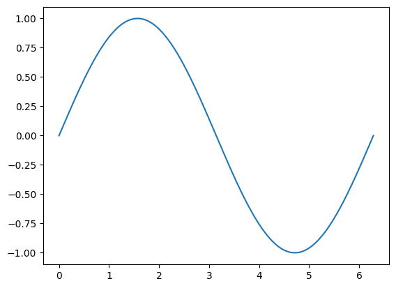
Let’s start with a minimal example here (following https://matplotlib.org/stable/users/getting_started/):

import matplotlib.pyplot as plt # import matplotlib, a conventional module name is plt
import numpy as np

x = np.linspace(0, 2 * np.pi, 200) # creates a NumPy array from 0 to 2pi, 200 equallys-paced points  
y = np.sin(x) # take the NumPy array and create another one, where each term is now the sine of each of the elements of the above NumPy array

fig, ax = plt.subplots() # create the elements required for matplotlib. This creates a figure containing a single set of axes.

ax.plot(x, y) # make a one-dimensional plot using the above arrays

plt.show() # show the plot here

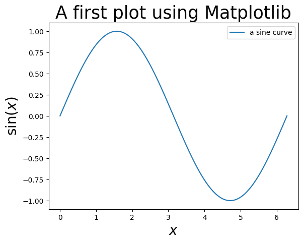
Let’s add a title, axis labels and a legend:

import matplotlib.pyplot as plt # import matplotlib, a conventional module name is plt
import numpy as np

x = np.linspace(0, 2 * np.pi, 200) # creates a NumPy array from 0 to 2pi, 200 equallys-paced points  
y = np.sin(x) # take the NumPy array and create another one, where each term is now the sine of each of the elements of the above NumPy array

fig, ax = plt.subplots() # create the elements required for matplotlib. This creates a figure containing a single axes.

# set the labels and titles:
ax.set_xlabel(r'$x$', fontsize=20) # set the x label
ax.set_ylabel(r'$\sin (x)$', fontsize=20) # set the y label. Note that the 'r' is necessary to remove the need for double slashes. You can use LaTeX! 
ax.set_title('A first plot using Matplotlib', fontsize=25) # set the title 

# make a one-dimensional plot using the above arrays, add a custom label
ax.plot(x, y, label='a sine curve') 

# construct the legend:
ax.legend(loc='upper right')  # Add a legend

plt.show() # show the plot here

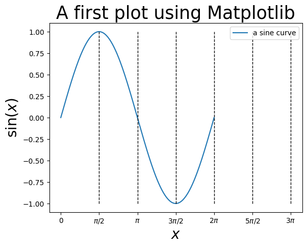
You can also change the labels of the axes to whatever you like, and plot vertical (or horizontal) lines:

import matplotlib.pyplot as plt # import matplotlib, a conventional module name is plt
import numpy as np
from math import pi

x = np.linspace(0, 2 * np.pi, 200) # creates a NumPy array from 0 to 2pi, 200 equallys-paced points  
y = np.sin(x) # take the NumPy array and create another one, where each term is now the sine of each of the elements of the above NumPy array

fig, ax = plt.subplots() # create the elements required for matplotlib. This creates a figure containing a single axes.

# set the labels and titles:
ax.set_xlabel(r'$x$', fontsize=20) # set the x label
ax.set_ylabel(r'$\sin (x)$', fontsize=20) # set the y label. Note that the 'r' is necessary to remove the need for double slashes. You can use LaTeX! 
ax.set_title('A first plot using Matplotlib', fontsize=25) # set the title 

# make a one-dimensional plot using the above arrays, add a custom label
ax.plot(x, y, label='a sine curve') 

# change the axis labels to correspond to [0, pi/2, pi, 1.5 * pi, 2*pi, 2.5*pi, 3*pi]
ax.set_xticks([0, pi/2, pi, 1.5 * pi, 2*pi, 2.5*pi, 3*pi])
ax.set_xticklabels(['0', '$\\pi/2$', '$\\pi$', '$3\\pi/2$', '$2\\pi$', '$5\\pi/2$', '$3\\pi$'])

# plot vertical lines at pi/2, pi, 3pi/2, 2pi, 5pi/2, 3pi
ax.vlines(x=pi/2, ymin=-1, ymax=1, linewidth=1, ls='--', color='black')
ax.vlines(x=pi, ymin=-1, ymax=1, linewidth=1, ls='--', color='black')
ax.vlines(x=3*pi/2, ymin=-1, ymax=1, linewidth=1, ls='--', color='black')
ax.vlines(x=2*pi, ymin=-1, ymax=1, linewidth=1, ls='--', color='black')
ax.vlines(x=2.5*pi, ymin=-1, ymax=1, linewidth=1, ls='--', color='black')
ax.vlines(x=3.0*pi, ymin=-1, ymax=1, linewidth=1, ls='--', color='black')

# construct the legend:
ax.legend(loc='upper right')  # Add a legend

plt.show() # show the plot here

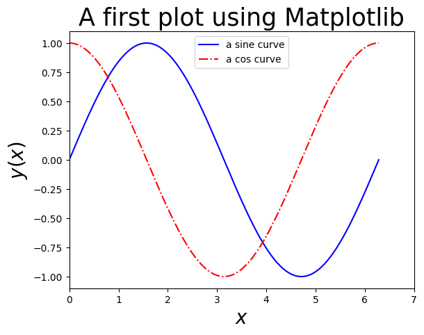
One can plot with different colors and linestyles. See https://matplotlib.org/stable/api/_as_gen/matplotlib.lines.Line2D.html#matplotlib.lines.Line2D.set_linestyle for linestyles and https://matplotlib.org/stable/users/explain/colors/colors.html for colors.

import matplotlib.pyplot as plt # import matplotlib, a conventional module name is plt
import numpy as np

x = np.linspace(0, 2 * np.pi, 200) # creates a NumPy array from 0 to 2pi, 200 equallys-paced points  
y = np.sin(x) # take the NumPy array and create another one, where each term is now the sine of each of the elements of the above NumPy array
z = np.cos(x) # also get a cosine 

fig, ax = plt.subplots() # create the elements required for matplotlib. This creates a figure containing a single axes.

# set the labels and titles:
ax.set_xlabel(r'$x$', fontsize=20) # set the x label
ax.set_ylabel(r'$y(x)$', fontsize=20) # set the y label
ax.set_title('A first plot using Matplotlib', fontsize=25) # set the title 

# set the x and y limits:
ax.set_xlim(0, 7)
ax.set_ylim(-1.1,1.1)

# make one-dimensional plots using the above arrays, add a custom label, linestyles and colors:
ax.plot(x, y, color='blue', linestyle='-', label='a sine curve') 
ax.plot(x, z, color='red', linestyle='-.', label='a cos curve') 

# construct the legend:
ax.legend(loc='upper center')  # Add a legend

plt.show() # show the plot here

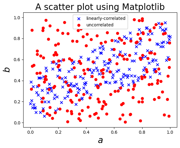
You can also create scatter plots! Here’s an example, where we generate a completely uncorrelated set and a slightly correlated set:

import matplotlib.pyplot as plt # import matplotlib, a conventional module name is plt
import numpy as np

x = np.linspace(0, 1, 200) # creates a NumPy array from 0 to 2pi, 200 equallys-paced points 
# Now suppose that we have random noise around the curve y = x: 
y = 0.5*(x+np.random.random(200)) # generates a NumPy array of size 200 with random floats in [0,1)

# now generate a completely uncorrelated sample of size 200 
z = np.random.random(200)
h = np.random.random(200)

fig, ax = plt.subplots() # create the elements required for matplotlib. This creates a figure containing a single axes.

# set the labels and titles:
ax.set_xlabel(r'$a$', fontsize=20) # set the x label
ax.set_ylabel(r'$b$', fontsize=20) # set the y label
ax.set_title('A scatter plot using Matplotlib', fontsize=20) # set the title 

# make one-dimensional plots using the above arrays, add a custom label, marker styles and colors:
ax.scatter(x, y, color='blue', marker='x', label='linearly-correlated') 
ax.scatter(z, h, color='red', marker='o',  label='uncorrelated') 

# construct the legend:
ax.legend(loc='upper center', framealpha=1.0)  # Add a legend, make it opaque

plt.show() # show the plot here

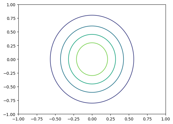
Matplotlib can also generate 2D plots, e.g. contours:

import matplotlib.pyplot as plt
import numpy as np

# make data: X and Y are defined over a 100x100 grid between (-1,1) in both dimensions. 
X, Y = np.meshgrid(np.linspace(-1, 1, 100), np.linspace(-1, 1, 100))

# now calculate a function over this grid, e.g.: 
Z = np.exp(-5*X**2) * np.exp(-2.5*Y**2)
levels = np.linspace(np.min(Z), np.max(Z), 6) # calculate six 'levels' on the contour

# plot
fig, ax = plt.subplots()

# make the contour:
ax.contour(X, Y, Z, levels=levels)

plt.show()

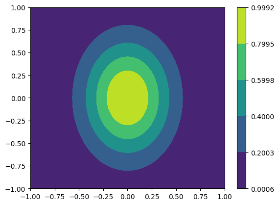
This can also be a “filled” contour, and you can add a color bar to help understand the contour:

import matplotlib.pyplot as plt
import numpy as np

# make data: X and Y are defined over a 100x100 grid between (-1,1) in both dimensions. 
X, Y = np.meshgrid(np.linspace(-1, 1, 100), np.linspace(-1, 1, 100))

# now calculate a function over this grid, e.g.: 
Z = np.exp(-5*X**2) * np.exp(-2.5*Y**2)
levels = np.linspace(np.min(Z), np.max(Z), 6) # calculate six 'levels' on the contour

# plot
fig, ax = plt.subplots()

# make the contour:
cs = ax.contourf(X, Y, Z, levels=levels)

# add a color bar:
cbar = fig.colorbar(cs)

plt.show()

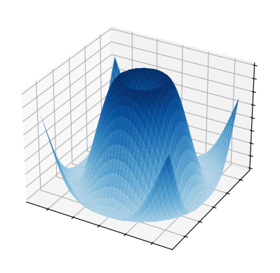
You can also plot in three-dimensions:

import matplotlib.pyplot as plt
import numpy as np

from matplotlib import cm

# Make data
X = np.arange(-5, 5, 0.25)
Y = np.arange(-5, 5, 0.25)
X, Y = np.meshgrid(X, Y) # You need the data to be defined over a grid 
R = np.sqrt(X**2 + Y**2)
Z = np.sin(R)

# Plot the surface
fig, ax = plt.subplots(subplot_kw={"projection": "3d"})
ax.plot_surface(X, Y, Z, vmin=Z.min() * 2, cmap=cm.Blues)

ax.set(xticklabels=[],
       yticklabels=[],
       zticklabels=[]) # remove tick labels

plt.show()

There’s tons of functionality in Matplotlib! For examples, check out: https://matplotlib.org/stable/plot_types/index.html and https://matplotlib.org/stable/gallery/index.html.

1.8.6. How to make good plots using matplotlib

Make sure your plots contain all the necessary ingredients. Some essential elements of a good graph are as follows:

• Ensure that the axes are correctly labeled, along with the units. E.g. if we are measuring the “Energy” variable in Joules along one axis, the label string should be: “Energy [J]”.

• A title is always helpful: e.g. “Energy versus Temperature”.

• You should include a legend which correctly labels what you are plotting. All lines should be included in the legend. Place the legend where it does not cover important data.

• Do not rely on color alone to distinguish curves. Pair color with line style and/or markers so the plot remains readable in grayscale and for color-vision deficiencies.

• Keep line widths consistent and readable (too thin disappears when exported; too thick can obscure data).

• Use sensible font sizes for axis labels, tick labels, title, and legend.

• Show uncertainty when it exists: error bars, shaded confidence bands, or standard deviation regions can be more informative than a single curve.

• Use gridlines selectively: light gridlines can help read values, but heavy grids often dominate the figure.

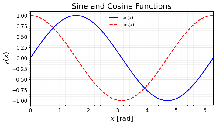
Use the following code as a template for your future graphs:

import matplotlib.pyplot as plt  # import matplotlib, a conventional module name is plt
import numpy as np

x = np.linspace(0, 2 * np.pi, 200)  # creates a NumPy array from 0 to 2pi, 200 equally spaced points
y = np.sin(x)  # sine evaluated on the array
z = np.cos(x)  # cosine evaluated on the array

# create the elements required for matplotlib. This creates a figure containing a single axes.
fig, ax = plt.subplots(figsize=(7, 4), constrained_layout=True)

# set the labels and titles (include units where appropriate):
ax.set_xlabel(r'$x$ [rad]', fontsize=16)     # set the x label
ax.set_ylabel(r'$y(x)$', fontsize=16)        # set the y label
ax.set_title('Sine and Cosine Functions', fontsize=18)  # set the title

# set the x and y limits:
ax.set_xlim(0, 2 * np.pi)
ax.set_ylim(-1.1, 1.1)

# make one-dimensional plots using the above arrays, add labels, line styles and colors:
ax.plot(x, y, color='blue', linestyle='-', linewidth=2, label=r'$\sin(x)$')
ax.plot(x, z, color='red', linestyle='--', linewidth=2, label=r'$\cos(x)$')

# optional: add a light grid to help read off values (without dominating the plot)
ax.grid(True, which='major', alpha=0.3)
ax.minorticks_on()
ax.grid(True, which='minor', alpha=0.15)

# make tick labels readable
ax.tick_params(axis='both', which='major', labelsize=12)

# construct the legend (avoid covering important data)
ax.legend(loc='upper center', frameon=False)

plt.show()  # show the plot here
# if you want to save the plot:
# filename = 'myplot.pdf'
# fig.savefig(filename, dpi=dpi, bbox_inches="tight")

1.9. Other Useful Modules

1.9.1. pandas

According to the pandas webpage: https://pandas.pydata.org

pandas is a fast, powerful, flexible and easy to use open source data analysis and manipulation tool, built on top of the Python programming language.

pandas is useful when working with tabular data, such as data stored in spreadsheets or databases. pandas can help you to explore, clean, and process your data. In pandas, a data table is called a DataFrame.

We will introduce some pandas functionality during the course.

1.9.2. PrettyTable

PrettyTable is “a simple Python library for easily displaying tabular data in a visually appealing ASCII table format”. (https://pypi.org/project/prettytable/).

Here’s an example:

from prettytable import PrettyTable

x = PrettyTable()
x.field_names = ["Particle Name", "Electric Charge", "Spin"]
x.add_row(["Electron", "-1", "1/2"])
x.add_row(["Photon", "0", "1"])
x.add_row(["Higgs Boson", "0", "1"])
x.add_row(["Positron", "+1", "1/2"])
x.add_row(["Graviton", "0", "2"])
print(x)

+---------------+-----------------+------+
| Particle Name | Electric Charge | Spin |
+---------------+-----------------+------+
|    Electron   |        -1       | 1/2  |
|     Photon    |        0        |  1   |
|  Higgs Boson  |        0        |  1   |
|    Positron   |        +1       | 1/2  |
|    Graviton   |        0        |  2   |
+---------------+-----------------+------+

1.9.3. tqdm

With tqdm you can instantly make your loops show a smart progress meter. e.g.:

from tqdm import tqdm
import time
for i in tqdm(range(20)):
    time.sleep(0.1)

  0%|                                                                                                                     | 0/20 [00:00<?, ?it/s]

  5%|█████▍                                                                                                       | 1/20 [00:00<00:01,  9.52it/s]

 10%|██████████▉                                                                                                  | 2/20 [00:00<00:01,  9.49it/s]

 15%|████████████████▎                                                                                            | 3/20 [00:00<00:01,  9.47it/s]

 20%|█████████████████████▊                                                                                       | 4/20 [00:00<00:01,  9.42it/s]

 25%|███████████████████████████▎                                                                                 | 5/20 [00:00<00:01,  9.52it/s]

 30%|████████████████████████████████▋                                                                            | 6/20 [00:00<00:01,  9.60it/s]

 35%|██████████████████████████████████████▏                                                                      | 7/20 [00:00<00:01,  9.50it/s]

 40%|███████████████████████████████████████████▌                                                                 | 8/20 [00:00<00:01,  9.43it/s]

 45%|█████████████████████████████████████████████████                                                            | 9/20 [00:00<00:01,  9.40it/s]

 50%|██████████████████████████████████████████████████████                                                      | 10/20 [00:01<00:01,  9.36it/s]

 55%|███████████████████████████████████████████████████████████▍                                                | 11/20 [00:01<00:00,  9.38it/s]

 60%|████████████████████████████████████████████████████████████████▊                                           | 12/20 [00:01<00:00,  9.36it/s]

 65%|██████████████████████████████████████████████████████████████████████▏                                     | 13/20 [00:01<00:00,  9.34it/s]

 70%|███████████████████████████████████████████████████████████████████████████▌                                | 14/20 [00:01<00:00,  9.34it/s]

 75%|█████████████████████████████████████████████████████████████████████████████████                           | 15/20 [00:01<00:00,  9.34it/s]

 80%|██████████████████████████████████████████████████████████████████████████████████████▍                     | 16/20 [00:01<00:00,  9.36it/s]

 85%|███████████████████████████████████████████████████████████████████████████████████████████▊                | 17/20 [00:01<00:00,  9.38it/s]

 90%|█████████████████████████████████████████████████████████████████████████████████████████████████▏          | 18/20 [00:01<00:00,  9.48it/s]

 95%|██████████████████████████████████████████████████████████████████████████████████████████████████████▌     | 19/20 [00:02<00:00,  9.45it/s]

100%|████████████████████████████████████████████████████████████████████████████████████████████████████████████| 20/20 [00:02<00:00,  9.55it/s]

100%|████████████████████████████████████████████████████████████████████████████████████████████████████████████| 20/20 [00:02<00:00,  9.43it/s]

1.9.4. SymPy

From the SymPy webpage (https://www.sympy.org/en/index.html):

SymPy is a Python library for symbolic mathematics. It aims to become a full-featured computer algebra system (CAS) while keeping the code as simple as possible in order to be comprehensible and easily extensible. SymPy is written entirely in Python.

Here’s an example of what SymPy can do:

from sympy import *
x, t, z, nu = symbols('x t z nu')

init_printing(use_unicode=True) 

# take the derivative of sin(x) * exp(x) wrt. x:
diff(sin(x)*exp(x), x)

integrate(exp(x)*sin(x) + exp(x)*cos(x), x) # integrate the above to get the function back!

# calculate the integral of sin(x**2) dx from -infinity to +infinity:
integrate(sin(x**2), (x, -oo, oo))

# find the limit of sin(x)/x as x->0:
limit(sin(x)/x, x, 0)

# solve the equation x**2 - 2 = 0 for x:
solve(x**2 - 2, x)

You can also output directly in LaTeX!

latex(Integral(cos(x)**2, (x, 0, pi)))

'\\int\\limits_{0}^{\\pi} \\cos^{2}{\\left(x \\right)}\\, dx'

init_printing(use_unicode=False) 

1.10. The Elephant in the room: Using Generative AI and LLMs

Generative Artificial Intelligence (AI) and Large Language Models (LLMs) are widely available and powerful tools. These tools can be used effectively in scientific research and learning.

There are several challenges to be aware when using these tools (see e.g. https://grad.uw.edu/advice/effective-and-responsible-use-of-ai-in-research/ for a more detailed overview):

• They can summarize material, but they are not always accurate or unbiased.

• The quality of the output depends on the algorithmic approach, the quality of the training data, and the user’s understanding of the tools’ limitations and biases as they write queries. Though the content generated may sound very plausible, it may be inaccurate such as including non-existent publications or incorrect citations of publications.

• People are prone to biases in their work, and AI can pick up those biases from the training data and even amplify them or introduce its own.

In research, AI can be a valuable tool for assistance but is not an accountable entity for the research outcomes since the ultimate responsibility of research lies with the human.

In this course, and in learning how to code, you are not strictly forbidden to use AI. These tools will be useful to you in your future careers. Use is allowed for debugging explanations and conceptual review, and not allowed to generate full solution code.

However, to facilitate your learning, you will have to use AI and LLMs as a tool, not as a substitute for thinking. Note that recent studies have shown that using LLMs can actually increase development time of code (see https://arxiv.org/pdf/2507.09089), but of course this is a subject of on-going research.

So here’s some advice for using AI/LLMs in solving computational problems in this course:

• Do not use AI/LLMs to solve the assignments directly. As previously mentioned in this chapter, programming is an art, and you have to get your hands dirty to become proficient in it. In this course, I suggest that you use AI/LLMs as a sort of last resort.

• When you begin working on your assignment take the following route:

  1. Think about the necessary steps to solve the problem. What is the algorithm that you need to use? Is there some code in the book that you can already rely on? If so, try and understand how it works and use it as a starting point.

  2. Write your reasoning in comments in the code directly (using #.

  3. Let’s assume that you have most of your program written down, but now you want to add something new to it. Before using an LLM, use a search engine to find, e.g. a manual for the code. These contain descriptions of how to use the functionality, and very often they contain concrete examples. Copy an example that you understand, and use it as a basis.

  4. If the example does not work as intended, or there is an error, use a search engine to search for the error.

  5. If the above fails, ask an LLM to give you information on the error and how you may solve the particular issue.

  6. If AI suggested something, you must validate it via: reading official docs, writing a minimal reproducible example, adding 1-2 unit tests, and checking edge cases.

To ensure the above points, you will need to add a disclosure at the start of each assignment. Some examples are:

• AI use statement: I used the AI tool <…> to understand what np.logspace does.

• AI use statement: I used the AI tool <…> to debug a for loop that kept giving me an error.

Even if you did not use AI, you will still need to add an AI statement:

• AI use statement: None