1. Hello Whimsical World of Pythonic Physics!

1.1. Making Computers Obey

1.1.1. Machine Language

Computers always do exactly as they are told! Instructions they understand are in a machine language.

But when writing and running programs, we communicate to the computer through “shells”, in high-level languages (e.g. Python, Java, Fortran, C, …), or through problem-solving environments (e.g. Maple, Mathematica, Matlab, …).

Eventually these commands/programs are translated into the basic machine language that the hardware understands.

1.1.2. Shells, Operating Systems and Compilers

A shell: is a command-line interpreter: a small set of programs run by a computer that respond to the commands that you key in. The job of th eshell is to run programs, compilers and utilities. A demonstration of this will be given during the lectures, but we won’t be using shells extensively!

Operating systems, e.g. Unix, DOS, Linux, MacOS, Windows, are a group of programs used by the computer to communicate with users and devices, to store and read data, and to execute programs.

When you submit a program to your computer in a high-level language, the computer uses a compiler to process it. The compiler translates your program into machine language.

Fortran and C (e.g.) read the entire program and then translate it into basic machine instructions. These are known as “compiled languages”.

BASIC/Maple translate each line of program as it is entered. These are “interpreted languages”.

Python and Java are a mix of both.

1.1.3. Programming Warmup

Here’s some “pseudocode” for a program that intends to calculate the area of a circle:

read radius # the input 
calculate area of circle # the numerics
print area # the output

To actually get the computer to do the numerics, we have to specify an algorithm. The pseudocode would then look like:

read radius # the input
PI = 3.14 # a constant
area = PI * r * r # the algorithm
print area # output

1.1.4. Structure and Reproducible Program Design

Programming is a written art that blends the elements of science, math, and computer science into a set of instructions that permit a computer to accomplish a desired task.

It is important that the source code of your program itself is available to others so that they can reproduce and extend your results!

Reproducibility is an essential ingredient in science.

In addition to the grammar of the computer language, a scientific program should include a number of essential elements to ensure the program’s validity and useability.

As with other arts, it is recommended that until you know better, you should follow some simple rules:

A good program should:

• give correct answers.

• be clear and easy to read, with the action of each part easy to analyze.

• document itself for the readers/programmer.

• be easy to use.

• be built out of small programs that can be independently verified.

• be easy to modify and robust enough to keep giving correct answers arfter modification and simple debugging.

• document the data fomats used.

• use trusted libraries.

• be published or passed onto others to use and to develop further.

An elementary way to make any program clear is to structure it with indentation, skipped lines, parentheses, all placed strategically.

Python uses indentation as a structure element, as well as for clarity.

1.2. Introduction to Python

From the Python tutorial: https://docs.python.org/3.12/tutorial/index.html

“Python is an easy to learn, powerful programming language.

It has efficient high-level data structures and a simple but effective approach to object-oriented programming.

Python’s elegant syntax and dynamic typing, together with its interpreted nature, make it an ideal language for scripting and rapid application development in many areas on most platforms.”

Today we will learn how to use Python in a jupyter notebook (such as this one) and use it to solve some basic problems, including visualization.

1.2.1. What is Python?

Python is an interpreted, interactive, object-oriented programming language. It incorporates modules, exceptions, dynamic typing, very high level dynamic data types, and classes.

1.2.2. Aside: Why is it called that?!

When he began implementing Python, Guido van Rossum was also reading the published scripts from “Monty Python’s Flying Circus”, a BBC comedy series from the 1970s. Van Rossum thought he needed a name that was short, unique, and slightly mysterious, so he decided to call the language Python.

1.2.3. Jupyter Notebooks, the Gitlab repository and Binder

There are many ways to use Python. We will explore some of them, but I will mainly be using jupyter notebooks, such as the one you are currently looking at. The easiest option is to use “binder” (https://mybinder.org/) in conjunction with the course code/notes repository: apapaefs/compphys.

Effectively, you can simply follow this link to open a jupyter lab: https://mybinder.org/v2/gl/apapaefs%2Fcompphys/HEAD.

You will find the environment you see here (if you are in class right now!), along with the course files.

1.2.4. Let’s write some code!

We can already write code in this notebook:

print("Hello Whimsical World of Pythonic Physics!")

Hello Whimsical World of Pythonic Physics!

Try it now! Congratulations! You’ve written your first program in Python!

Let’s now define some variables:

eggs = 3
text1 = "Break the"
text2 = "eggs" # comments are written this way in Python

You can use Python as a calculator:

2 + 3

5

2 * 42

84

8/5

1.6

Note that the above is a float of double precision! (see later)

3**2

9

And you can use variables during these operations:

eggs * 2

6

It’s very easy to manipulate text in Python (represented by “strings”). You can define strings as above, either in “” or ‘’.

text3 = text1 + “ “ + str(eggs) + “ “ + text2 print(text3)

Strings can be indexed:

text3[0]

---------------------------------------------------------------------------
NameError                                 Traceback (most recent call last)
Cell In[8], line 1
----> 1 text3[0]

NameError: name 'text3' is not defined

text3[1]

'r'

text3 = [1, 4, 9, 16, 25]

Negative integers start counting from the right:

text3[-1]

's'

text3[-2]

'g'

You can also “slice” strings:

text3[0:2]  # characters from position 0 (included) to 2 (excluded)

'Br'

text3[2:5]  # characters from position 2 (included) to 5 (excluded)

'eak'

text3[4:]   # characters from position 4 (included) to the end

'k the 3 eggs'

len() tells you how long a string is:

len(text3)

16

Lists are used to group together values. They are written as a list of comma-separated values (items) between square brackets. They may contain items of different types but usually the items all have the same type.

squares = [1, 4, 9, 16, 25]

Like strings, lists can be indexed and sliced:

squares[3]  # indexing returns the item

16

squares[-1] # indexing returns the last item

25

squares[1:] # returns the second element up to the end

[4, 9, 16, 25]

Lists also support operations like concatenation:

squares + [36, 49, 64, 81, 100]

[1, 4, 9, 16, 25, 36, 49, 64, 81, 100]

Unlike strings, which are immutable, lists are a mutable type, i.e. it is possible to change their content:

cubes = [1, 8, 27, 65, 125]  # something's wrong here
4 ** 3  # the cube of 4 is 64, not 65!

64

cubes[3] = 64  # replace the wrong value
cubes

[1, 8, 27, 64, 125]

You can also add new items at the end of the list, by using the list.append() method:

cubes.append(216)  # add the cube of 6
cubes.append(7 ** 3)  # and the cube of 7
cubes

[1, 8, 27, 64, 125, 216, 343]

len() also applies to lists:

len(cubes)

7

Let’s use Python to write down the first few terms in the Fobonacci series:

# Fibonacci series:
# the sum of two elements defines the next
a = 0
b = 1 # define the first two
while a < 10: # do this while the number a is less than 10, stop when it exceeds 10.
    print(a) # print the next number in the series
    c = b
    b = a+c # a becomes the next number to be printed, and calculate the one after that.
    a = c

0
1
1
2
3
5
8

1.3. Control Flow Tools

1.3.1. if Statements

One of the most well-known statement type is the if statement. An example:

x = int(input("Please enter an integer: "))

if x < 0: 
    x = 0
    print('Negative integer detected, changed to zero!')
elif x == 0:
    print("Zero")
elif x == 1:
    print("One")
else: 
    print("Positive integer, not one")

Negative integer detected, changed to zero!

‘elif’ is short for ‘else if’, there can be any number of such statements (including none). ‘else’ is optional and is ‘triggered’ if all other statements are not satisfied.

1.3.2. for Statements

Python’s for statement iterates over the items of any sequence (e.g. a list or a string), in the order they appear in the sequence. E.g.:

# measure the length of all the strings in a list:
words = ['Einstein', 'Galileo', 'Copernicus']
for w in words:
    print(w, len(w))

Einstein 8
Galileo 7
Copernicus 10

If instead you want to iterate over the sequence of numbers, thne range() function comes in handy:

for i in range(3):
    print(words[i], len(words[i]))

Einstein 8
Galileo 7
Copernicus 10

or, equivalently:

for i in range(len(words)):
    print(i, words[i], len(words[i]))

0 Einstein 8
1 Galileo 7
2 Copernicus 10

1.3.3. break and continue Statements, and else Clauses on Loops

The break statement breaks out the innermost enclosing for or while loop. E.g.:

for w in words:
    if w == 'Galileo':
        continue
    print(w)

Einstein
Copernicus

A for or while loop can include an else clause. In a for loop the else clause is executed after the loop reaches its final iteration. In a while loop, it’s executed after the loop’s condition becomes false. In either kind of loop, the else clause is not executed if the loop was terminated by a break.

In the following example, an else clause is used at the end of a for loop which contains an if statement that checks whether a number is divisible by all numbers smaller than itself. (The n % x part calculates the remainder of the division n/x).

for n in range(2,10):
    for x in range(2, n):
        if n%x==0:
            print(n, 'equals', x, '*', n/x)
            break # we have found a number smaller than n is a factor of n, so n is not a prime number! -> break the for loop here -> else is not executed!
    else: 
        # loop fell through without finding a factor 
        print(n, 'is a prime number')

2 is a prime number
3 is a prime number
4 equals 2 * 2.0
5 is a prime number
6 equals 2 * 3.0
7 is a prime number
8 equals 2 * 4.0
9 equals 3 * 3.0

The continue statement continues with the next iteration of the loop:

for num in range(2, 10):
    if num % 2 == 0:
        print("Found an even number", num)
        continue
    print("Found an odd number", num)

Found an even number 2
Found an odd number 3
Found an even number 4
Found an odd number 5
Found an even number 6
Found an odd number 7
Found an even number 8
Found an odd number 9

1.4. Defining Functions

We can create a function that writes the Fibonacci series to an arbitrary boundary:

def fib(n):    # write Fibonacci series up to n
    """Print a Fibonacci series up to n."""
    a, b = 0, 1
    while a < n:
        print(a, end=' ')
        a, b = b, a+b

The keyword def introduces a function definition. It must be followed by the function name and the parenthesized list of formal parameters. The statements that form the body of the function start at the next line, and must be indented. The first statement of the function body can optionally be a string literal; this string literal is the function’s documentation string.

We can execute the function by calling it with a parameter, e.g.:

fib(2000)

0 1 1 2 3 5 8 13 21 34 55 89 144 233 377 610 987 1597 

Functions without return statements return None:

print(fib(2000))

0 1 1 2 3 5 8 13 21 34 55 89 144 233 377 610 987 1597 None

We can instead create a function that returns the values we are after, e.g. in a list:

def fib2(n):  # return Fibonacci series up to n
    """Return a list containing the Fibonacci series up to n."""
    result = []
    a, b = 0, 1
    while a < n:
        result.append(a)    # see below
        a, b = b, a+b
    return result

And we can call it to create a list, e.g. fib100:

f100 = fib2(100)

print(f100)

[0, 1, 1, 2, 3, 5, 8, 13, 21, 34, 55, 89]

Note that append is a method that acts on the list object result to add a new element at its end.

For more details on defining functions, see https://docs.python.org/3/tutorial/controlflow.html#more-on-defining-functions. We will discuss some of those aspects where necessary during the course.

1.5. Data Structures

1.5.1. List Methods

We already mentionewd the list.append() method for a list. The list data type has some more methods, some of which are:

• list.append(x): Add an item to the end of the list. Equivalent to a[len(a):] = [x].

• list.insert(i, x): Insert an item at a given position. The first argument is the index of the element before which to insert, so a.insert(0, x) inserts at the front of the list, and a.insert(len(a), x) is equivalent to a.append(x).

• list.remove(x): Remove the first item from the list whose value is equal to x. It raises a ValueError if there is no such item.

• list.pop([i]): Remove the item at the given position in the list, and return it. If no index is specified, a.pop() removes and returns the last item in the list. (The square brackets around the i in the method signature denote that the parameter is optional, not that you should type square brackets at that position. You will see this notation frequently in the Python Library Reference.)

• list.clear(): Remove all items from the list.

• list.count(x): Return the number of times x appears in the list.

• list.reverse(): Reverse the elements of the list in place.

• list.sort(*, key=None, reverse=False): Sort the items of the list in place (the arguments can be used for sort customization, see sorted() for their explanation).

• list.reverse(): Reverse the elements of the list in place.

• list.copy(): Return a shallow copy of the list. Equivalent to a[:].

The following examples use several of the list methods:

fruits = ['orange', 'apple', 'pear', 'banana', 'kiwi', 'apple', 'banana']

fruits.count('apple')

2

fruits.count('tangerine')

0

fruits.index('banana')

3

fruits.index('banana', 4)  # Find next banana starting at position 4

6

fruits.reverse()
fruits

['banana', 'apple', 'kiwi', 'banana', 'pear', 'apple', 'orange']

fruits.append('grape')
fruits

['banana', 'apple', 'kiwi', 'banana', 'pear', 'apple', 'orange', 'grape']

fruits.sort()
fruits

['apple', 'apple', 'banana', 'banana', 'grape', 'kiwi', 'orange', 'pear']

fruits.pop()

'pear'

1.5.2. List Comprehensions

List comprehensions provide a concise way to create lists. Common applications are to make new lists where each element is the result of some operations applied to each member of another sequence or iterable, or to create a subsequence of those elements that satisfy a certain condition.

E.g. let’s assume we want to create a list of squares, like:

squares = []
for x in range(10):
    squares.append(x**2)
squares

[0, 1, 4, 9, 16, 25, 36, 49, 64, 81]

We can instead use a list comprehension:

squares = [x**2 for x in range(10)]
squares

[0, 1, 4, 9, 16, 25, 36, 49, 64, 81]

A list comprehension consists of brackets containing an expression followed by a for clause, then zero or more for or if clauses. The result will be a new list resulting from evaluating the expression in the context of the for and if clauses which follow it.

E.g. Let’s say we want the even numbers in the squares list:

even_squares = [y for y in squares if y%2 == 0]
even_squares

[0, 4, 16, 36, 64]

1.5.3. Tuples and Sequences

We saw that lists and strings have many common properties, such as indexing and slicing operations. They are two examples of sequence data types (see Sequence Types — list, tuple, range). There is also another standard sequence data type: the tuple.

A tuple consists of a number of values separated by commas, for instance:

t = 12345, 54321, 'hello!'
t[0]

12345

# Tuples may be nested:
u = t, (1, 2, 3, 4, 5)
u

((12345, 54321, 'hello!'), (1, 2, 3, 4, 5))

As you see, on output tuples are always enclosed in parentheses, so that nested tuples are interpreted correctly; they may be input with or without surrounding parentheses, although often parentheses are necessary anyway (if the tuple is part of a larger expression). It is not possible to assign to the individual items of a tuple, however it is possible to create tuples which contain mutable objects, such as lists.

Though tuples may seem similar to lists, they are often used in different situations and for different purposes. Tuples are immutable, and usually contain a heterogeneous sequence of elements that are accessed via unpacking (see later) or indexing. Lists are mutable, and their elements are usually homogeneous and are accessed by iterating over the list.

# Tuples are immutable:
t[0] = 88888

---------------------------------------------------------------------------
TypeError                                 Traceback (most recent call last)
Cell In[94], line 2
      1 # Tuples are immutable:
----> 2 t[0] = 88888

TypeError: 'tuple' object does not support item assignment

1.5.4. Dictionaries

Another useful data type built into Python is the dictionary. Unlike sequences, which are indexed by a range of numbers, dictionaries are indexed by keys, which can be any immutable type; strings and numbers can always be keys. Tuples can be used as keys if they contain only strings, numbers, or tuples; if a tuple contains any mutable object either directly or indirectly, it cannot be used as a key. You can’t use lists as keys, since lists can be modified in place using index assignments, slice assignments, or methods like append() and extend().

It is best to think of a dictionary as a set of key: value pairs, with the requirement that the keys are unique (within one dictionary). A pair of braces creates an empty dictionary: {}. Placing a comma-separated list of key:value pairs within the braces adds initial key:value pairs to the dictionary; this is also the way dictionaries are written on output.

The main operations on a dictionary are storing a value with some key and extracting the value given the key. It is also possible to delete a key:value pair with del. If you store using a key that is already in use, the old value associated with that key is forgotten. It is an error to extract a value using a non-existent key.

Performing list(d) on a dictionary returns a list of all the keys used in the dictionary, in insertion order (if you want it sorted, just use sorted(d) instead). To check whether a single key is in the dictionary, use the in keyword.

Here is a small example using a dictionary:

tel = {'jack': 4098, 'sape': 4139}
tel['guido'] = 4127
tel

{'jack': 4098, 'sape': 4139, 'guido': 4127}

tel['jack']

4098

del tel['sape']
tel['irv'] = 4127
tel

{'jack': 4098, 'guido': 4127, 'irv': 4127}

list(tel)

['jack', 'guido', 'irv']

sorted(tel)

['guido', 'irv', 'jack']

'guido' in tel

True

'jack' not in tel

False

The dict() constructor builds dictionaries directly from sequences of key-value pairs:

dict([('sape', 4139), ('guido', 4127), ('jack', 4098)])

{'sape': 4139, 'guido': 4127, 'jack': 4098}

In addition, dict comprehensions can be used to create dictionaries from arbitrary key and value expressions:

{x: x**2 for x in (2, 4, 6)}

{2: 4, 4: 16, 6: 36}

When the keys are simple strings, it is sometimes easier to specify pairs using keyword arguments:

dict(sape=4139, guido=4127, jack=4098)

{'sape': 4139, 'guido': 4127, 'jack': 4098}

1.5.5. Looping Techniques

When looping through dictionaries, the key and corresponding value can be retrieved at the same time using the items() method:

knights = {'gallahad': 'the pure', 'robin': 'the brave'}
for k, v in knights.items():
    print(k, v)

gallahad the pure
robin the brave

When looping through a sequence, the position index and corresponding value can be retrieved at the same time using the enumerate() function.

for i, v in enumerate(['tic', 'tac', 'toe']):
    print(i, v)

0 tic
1 tac
2 toe

To loop over two or more sequences at the same time, the entries can be paired with the zip() function.

questions = ['name', 'quest', 'favorite color']
answers = ['lancelot', 'the holy grail', 'blue']
for q, a in zip(questions, answers):
    print('What is your {0}?  It is {1}.'.format(q, a))

What is your name?  It is lancelot.
What is your quest?  It is the holy grail.
What is your favorite color?  It is blue.

To loop over a sequence in sorted order, use the sorted() function which returns a new sorted list while leaving the source unaltered.

basket = ['apple', 'orange', 'apple', 'pear', 'orange', 'banana']
for i in sorted(basket):
    print(i)

apple
apple
banana
orange
orange
pear

Using set() on a sequence eliminates duplicate elements. The use of sorted() in combination with set() over a sequence is an idiomatic way to loop over unique elements of the sequence in sorted order.

basket = ['apple', 'orange', 'apple', 'pear', 'orange', 'banana']
for f in sorted(set(basket)):
    print(f)

apple
banana
orange
pear

1.6. Modules

1.6.1. User-Defined Modules

If you quit from the Python interpreter and enter it again, the definitions you have made (functions and variables) are lost. The same happens when you open a new jupyter notebook. Therefore, if you want to write a somewhat longer program, you are better off using a text editor to prepare the input for the interpreter and running it with that file as input instead. This is known as creating a script. As your program gets longer, you may want to split it into several files for easier maintenance. You may also want to use a handy function that you’ve written in several programs without copying its definition into each program.

To support this, Python has a way to put definitions in a file and use them in a script or in an interactive instance of the interpreter. Such a file is called a module; definitions from a module can be imported into other modules or into the main module (the collection of variables that you have access to in a script executed at the top level and in calculator mode).

A module is a file containing Python definitions and statements. The file name is the module name with the suffix .py appended. Within a module, the module’s name (as a string) is available as the value of the global variable __name__. For instance, we have created a file called fibo.py in the current directory with the following contents:

# Fibonacci numbers module

def fib(n):    # write Fibonacci series up to n
    a, b = 0, 1
    while a < n:
        print(a, end=' ')
        a, b = b, a+b
    print()

def fib2(n):   # return Fibonacci series up to n
    result = []
    a, b = 0, 1
    while a < n:
        result.append(a)
        a, b = b, a+b
    return result

Let’s import this module:

import fibo

This does not add the names of the functions defined in fibo directly to the current namespace; it only adds the module name fibo there. Using the module name you can access the functions:

fibo.fib(1000)

0 1 1 2 3 5 8 13 21 34 55 89 144 233 377 610 987 

fibo.fib2(100)

[0, 1, 1, 2, 3, 5, 8, 13, 21, 34, 55, 89]

fibo.__name__

'fibo'

There is a variant of the import statement that imports names from a module directly into the importing module’s namespace. For example:

from fibo import fib, fib2
fib(500)

0 1 1 2 3 5 8 13 21 34 55 89 144 233 377 

There is even a variant to import all names that a module defines:

from fibo import *
fib(500)

0 1 1 2 3 5 8 13 21 34 55 89 144 233 377 

If the module name is followed by as, then the name following as is bound directly to the imported module. This is effectively importing the module in the same way that import fibo will do, with the only difference of it being available as fib.

import fibo as fib
fib.fib(500)

0 1 1 2 3 5 8 13 21 34 55 89 144 233 377 

It can also be used when utilising ```from``` with similar effects:

from fibo import fib as fibonacci
fibonacci(500)

0 1 1 2 3 5 8 13 21 34 55 89 144 233 377 

1.6.2. Standard Modules and the Standard Library

Python comes with a library of standard modules, described in a separate document, the Python Library Reference (“Library Reference” hereafter). The built-in function dir() is used to find out which names a module defines. It returns a sorted list of strings:

import fibo
dir(fibo)

['__builtins__',
 '__cached__',
 '__doc__',
 '__file__',
 '__loader__',
 '__name__',
 '__package__',
 '__spec__',
 'fib',
 'fib2']

For a longer introduction to the standard library, check out: https://docs.python.org/3/tutorial/stdlib.html. Here, we will go through a few basic modules, and we will introduce more during the course.

The math module gives access to the underlying C library functions for floating point math:

import math
math.cos(math.pi / 4)

0.7071067811865476

math.log(1024, 2)

10.0

The random module provides tools for making random selections:

import random
random.choice(['apple', 'pear', 'banana'])

'banana'

random.sample(range(100), 10)   # sampling without replacement

[95, 54, 74, 84, 9, 25, 0, 8, 94, 49]

random.random()    # random float

0.004938036800039014

random.randrange(6) 

5

The statistics module calculates basic statistical properties (the mean, median, variance, etc.) of numeric data:

import statistics
data = [2.75, 1.75, 1.25, 0.25, 0.5, 1.25, 3.5]
print(statistics.mean(data))
print(statistics.median(data))
print(statistics.variance(data))

1.6071428571428572
1.25
1.3720238095238095

1.6.3. NumPy

NumPy is the fundamental package for scientific computing in Python. It is a Python library that provides a multidimensional array object, various derived objects (such as masked arrays and matrices), and an assortment of routines for fast operations on arrays, including mathematical, logical, shape manipulation, sorting, selecting, I/O, discrete Fourier transforms, basic linear algebra, basic statistical operations, random simulation and much more.

To access NumPy and its functions import it:

import numpy as np

Python lists vs NumPy arrays:

NumPy gives you an enormous range of fast and efficient ways of creating arrays and manipulating numerical data inside them. While a Python list can contain different data types within a single list, all of the elements in a NumPy array should be homogeneous. The mathematical operations that are meant to be performed on arrays would be extremely inefficient if the arrays weren’t homogeneous.

NumPy arrays are faster and more compact than Python lists. An array consumes less memory and is convenient to use. NumPy uses much less memory to store data and it provides a mechanism of specifying the data types. This allows the code to be optimized even further.

One way we can initialize NumPy arrays is from Python lists, using nested lists for two- or higher-dimensional data.

a = np.array([1, 2, 3, 4, 5, 6])

The elements can be accessed in the same way as lists, e.g.:

print(a[0])

1

You can add the arrays together with the plus sign.

data = np.array([1, 2])
ones = np.ones(2, dtype=int)
data + ones

array([2, 3])

You can, of course, do more than just addition!

data - ones

array([0, 1])

data * data

array([1, 4])

data / data

array([1., 1.])

Basic operations are simple with NumPy. If you want to find the sum of the elements in an array, you’d use sum(). This works for 1D arrays, 2D arrays, and arrays in higher dimensions.

a = np.array([1, 2, 3, 4])
a.sum()

10

There are times when you might want to carry out an operation between an array and a single number (also called an operation between a vector and a scalar) or between arrays of two different sizes:

data = np.array([1.0, 2.0])
data * 1.6

array([1.6, 3.2])

With NumPy you can create and manipulate matrices, generate random numbers, and much more! We will discuss specific applications during the course, but see https://numpy.org/doc/stable/index.html for detailed documentation.

1.6.4. SciPy

SciPy provides algorithms for optimization, integration, interpolation, eigenvalue problems, algebraic equations, differential equations, statistics and many other classes of problems. It is built on NumPy . It adds significant power to Python by providing the user with high-level commands and classes for manipulating and visualizing data.

Some subpackages of interest to physics are:

• Physical and mathematical constants (scipy.constants)

• Special functions (scipy.special)

• Integration (scipy.integrate)

• Optimization (scipy.interpolate)

• Fourier transforms (scipy.fft)

• Signal processing (scipy.signal)

• Linear Algebra (scipy.linalg)

• Spatial data structures and algorithms (scipy.spatial)

See https://docs.scipy.org/doc/scipy/tutorial/index.html#subpackages for the full list of subpackages.

Some examples:

import scipy
from scipy import constants, special, integrate

scipy.constants.speed_of_light # get the speed of light

# Compute the first ten zeros of integer-order Bessel functions Jn.
scipy.special.jn_zeros(2,10)

array([ 5.1356223 ,  8.41724414, 11.61984117, 14.79595178, 17.95981949,
       21.11699705, 24.27011231, 27.42057355, 30.5692045 , 33.71651951])

# Calculate the definite integral of sinx/x in [0,1]
scipy.integrate.quad(lambda x: np.sin(x)/x, 0, 1)

(0.946083070367183, 1.0503632079297087e-14)

1.6.5. Matplotlib (Plotting)

“If I can’t picture it, I can’t understand it.” - Albert Einstein

From the Matplotlib page: https://matplotlib.org:

Matplotlib is a comprehensive library for creating static, animated, and interactive visualizations in Python. Matplotlib makes easy things easy and hard things possible.

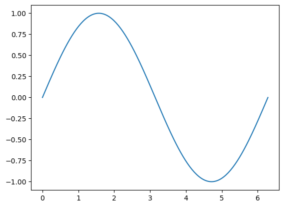
Let’s start with a minimal example here (following https://matplotlib.org/stable/users/getting_started/):

import matplotlib.pyplot as plt # import matplotlib, a conventional module name is plt
import numpy as np

x = np.linspace(0, 2 * np.pi, 200) # creates a NumPy array from 0 to 2pi, 200 equallys-paced points  
y = np.sin(x) # take the NumPy array and create another one, where each term is now the sine of each of the elements of the above NumPy array

fig, ax = plt.subplots() # create the elements required for matplotlib. This creates a figure containing a single set of axes.

ax.plot(x, y) # make a one-dimensional plot using the above arrays

plt.show() # show the plot here

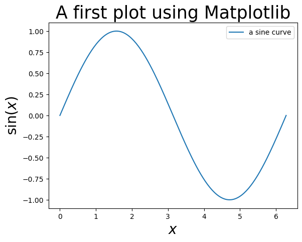
Let’s add a title, axis labels and a legend:

import matplotlib.pyplot as plt # import matplotlib, a conventional module name is plt
import numpy as np

x = np.linspace(0, 2 * np.pi, 200) # creates a NumPy array from 0 to 2pi, 200 equallys-paced points  
y = np.sin(x) # take the NumPy array and create another one, where each term is now the sine of each of the elements of the above NumPy array

fig, ax = plt.subplots() # create the elements required for matplotlib. This creates a figure containing a single axes.

# set the labels and titles:
ax.set_xlabel(r'$x$', fontsize=20) # set the x label
ax.set_ylabel(r'$\sin (x)$', fontsize=20) # set the y label. Note that the 'r' is necessary to remove the need for double slashes. You can use LaTeX! 
ax.set_title('A first plot using Matplotlib', fontsize=25) # set the title 

# make a one-dimensional plot using the above arrays, add a custom label
ax.plot(x, y, label='a sine curve') 

# construct the legend:
ax.legend(loc='upper right')  # Add a legend

plt.show() # show the plot here

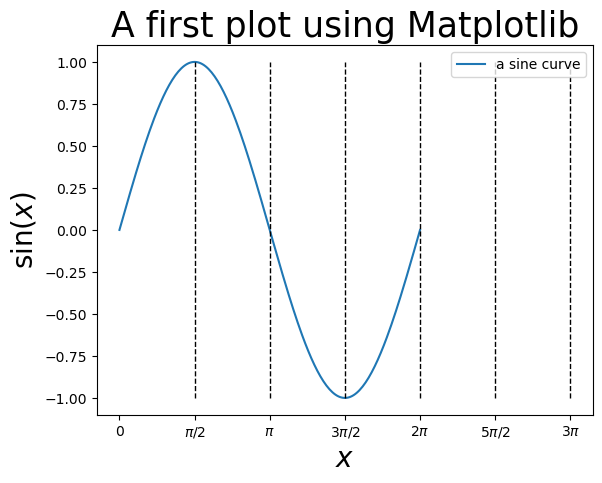
You can also change the labels of the axes to whatever you like, and plot vertical (or horizontal) lines:

import matplotlib.pyplot as plt # import matplotlib, a conventional module name is plt
import numpy as np
from math import pi

x = np.linspace(0, 2 * np.pi, 200) # creates a NumPy array from 0 to 2pi, 200 equallys-paced points  
y = np.sin(x) # take the NumPy array and create another one, where each term is now the sine of each of the elements of the above NumPy array

fig, ax = plt.subplots() # create the elements required for matplotlib. This creates a figure containing a single axes.

# set the labels and titles:
ax.set_xlabel(r'$x$', fontsize=20) # set the x label
ax.set_ylabel(r'$\sin (x)$', fontsize=20) # set the y label. Note that the 'r' is necessary to remove the need for double slashes. You can use LaTeX! 
ax.set_title('A first plot using Matplotlib', fontsize=25) # set the title 

# make a one-dimensional plot using the above arrays, add a custom label
ax.plot(x, y, label='a sine curve') 

# change the axis labels to correspond to [0, pi/2, pi, 1.5 * pi, 2*pi, 2.5*pi, 3*pi]
ax.set_xticks([0, pi/2, pi, 1.5 * pi, 2*pi, 2.5*pi, 3*pi])
ax.set_xticklabels(['0', '$\\pi/2$', '$\\pi$', '$3\\pi/2$', '$2\\pi$', '$5\\pi/2$', '$3\\pi$'])

# plot vertical lines at pi/2, pi, 3pi/2, 2pi, 5pi/2, 3pi
ax.vlines(x=pi/2, ymin=-1, ymax=1, linewidth=1, ls='--', color='black')
ax.vlines(x=pi, ymin=-1, ymax=1, linewidth=1, ls='--', color='black')
ax.vlines(x=3*pi/2, ymin=-1, ymax=1, linewidth=1, ls='--', color='black')
ax.vlines(x=2*pi, ymin=-1, ymax=1, linewidth=1, ls='--', color='black')
ax.vlines(x=2.5*pi, ymin=-1, ymax=1, linewidth=1, ls='--', color='black')
ax.vlines(x=3.0*pi, ymin=-1, ymax=1, linewidth=1, ls='--', color='black')

# construct the legend:
ax.legend(loc='upper right')  # Add a legend

plt.show() # show the plot here

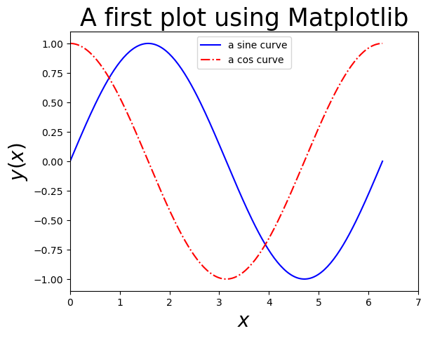
One can plot with different colors and linestyles. See https://matplotlib.org/stable/api/_as_gen/matplotlib.lines.Line2D.html#matplotlib.lines.Line2D.set_linestyle for linestyles and https://matplotlib.org/stable/users/explain/colors/colors.html for colors.

import matplotlib.pyplot as plt # import matplotlib, a conventional module name is plt
import numpy as np

x = np.linspace(0, 2 * np.pi, 200) # creates a NumPy array from 0 to 2pi, 200 equallys-paced points  
y = np.sin(x) # take the NumPy array and create another one, where each term is now the sine of each of the elements of the above NumPy array
z = np.cos(x) # also get a cosine 

fig, ax = plt.subplots() # create the elements required for matplotlib. This creates a figure containing a single axes.

# set the labels and titles:
ax.set_xlabel(r'$x$', fontsize=20) # set the x label
ax.set_ylabel(r'$y(x)$', fontsize=20) # set the y label
ax.set_title('A first plot using Matplotlib', fontsize=25) # set the title 

# set the x and y limits:
ax.set_xlim(0, 7)
ax.set_ylim(-1.1,1.1)

# make one-dimensional plots using the above arrays, add a custom label, linestyles and colors:
ax.plot(x, y, color='blue', linestyle='-', label='a sine curve') 
ax.plot(x, z, color='red', linestyle='-.', label='a cos curve') 

# construct the legend:
ax.legend(loc='upper center')  # Add a legend

plt.show() # show the plot here

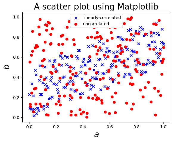
You can also create scatter plots! Here’s an example, where we generate a completely uncorrelated set and a slightly correlated set:

import matplotlib.pyplot as plt # import matplotlib, a conventional module name is plt
import numpy as np

x = np.linspace(0, 1, 200) # creates a NumPy array from 0 to 2pi, 200 equallys-paced points 
# Now suppose that we have random noise around the curve y = x: 
y = 0.5*(x+np.random.random(200)) # generates a NumPy array of size 200 with random floats in [0,1)

# now generate a completely uncorrelated sample of size 200 
z = np.random.random(200)
h = np.random.random(200)

fig, ax = plt.subplots() # create the elements required for matplotlib. This creates a figure containing a single axes.

# set the labels and titles:
ax.set_xlabel(r'$a$', fontsize=20) # set the x label
ax.set_ylabel(r'$b$', fontsize=20) # set the y label
ax.set_title('A scatter plot using Matplotlib', fontsize=20) # set the title 

# make one-dimensional plots using the above arrays, add a custom label, marker styles and colors:
ax.scatter(x, y, color='blue', marker='x', label='linearly-correlated') 
ax.scatter(z, h, color='red', marker='o',  label='uncorrelated') 

# construct the legend:
ax.legend(loc='upper center', framealpha=1.0)  # Add a legend, make it opaque

plt.show() # show the plot here

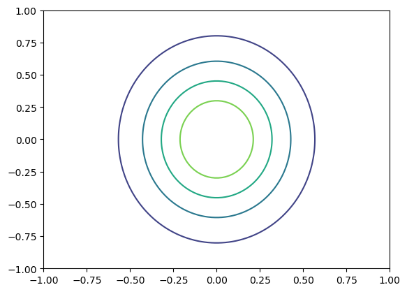
Matplotlib can also generate 2D plots, e.g. contours:

import matplotlib.pyplot as plt
import numpy as np

# make data: X and Y are defined over a 100x100 grid between (-1,1) in both dimensions. 
X, Y = np.meshgrid(np.linspace(-1, 1, 100), np.linspace(-1, 1, 100))

# now calculate a function over this grid, e.g.: 
Z = np.exp(-5*X**2) * np.exp(-2.5*Y**2)
levels = np.linspace(np.min(Z), np.max(Z), 6) # calculate six 'levels' on the contour

# plot
fig, ax = plt.subplots()

# make the contour:
ax.contour(X, Y, Z, levels=levels)

plt.show()

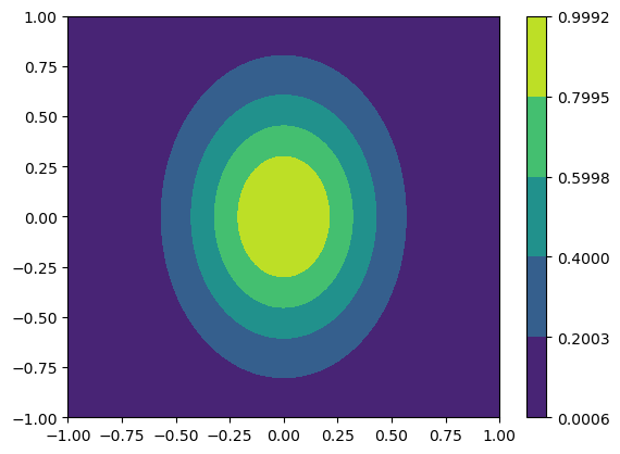
This can also be a “filled” contour, and you can add a color bar to help understand the contour:

import matplotlib.pyplot as plt
import numpy as np

# make data: X and Y are defined over a 100x100 grid between (-1,1) in both dimensions. 
X, Y = np.meshgrid(np.linspace(-1, 1, 100), np.linspace(-1, 1, 100))

# now calculate a function over this grid, e.g.: 
Z = np.exp(-5*X**2) * np.exp(-2.5*Y**2)
levels = np.linspace(np.min(Z), np.max(Z), 6) # calculate six 'levels' on the contour

# plot
fig, ax = plt.subplots()

# make the contour:
cs = ax.contourf(X, Y, Z, levels=levels)

# add a color bar:
cbar = fig.colorbar(cs)

plt.show()

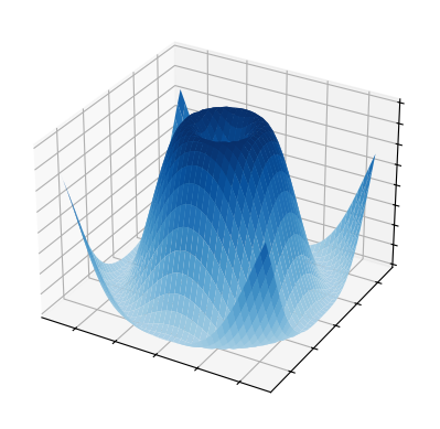
You can also plot in three-dimensions:

import matplotlib.pyplot as plt
import numpy as np

from matplotlib import cm

# Make data
X = np.arange(-5, 5, 0.25)
Y = np.arange(-5, 5, 0.25)
X, Y = np.meshgrid(X, Y) # You need the data to be defined over a grid 
R = np.sqrt(X**2 + Y**2)
Z = np.sin(R)

# Plot the surface
fig, ax = plt.subplots(subplot_kw={"projection": "3d"})
ax.plot_surface(X, Y, Z, vmin=Z.min() * 2, cmap=cm.Blues)

ax.set(xticklabels=[],
       yticklabels=[],
       zticklabels=[]) # remove tick labels

plt.show()

There’s tons of functionality in Matplotlib! For examples, check out: https://matplotlib.org/stable/plot_types/index.html and https://matplotlib.org/stable/gallery/index.html.

1.6.6. Other Useful Modules

1.6.6.1. pandas

According to the pandas webpage: https://pandas.pydata.org

pandas is a fast, powerful, flexible and easy to use open source data analysis and manipulation tool, built on top of the Python programming language.

pandas is useful when working with tabular data, such as data stored in spreadsheets or databases. pandas can help you to explore, clean, and process your data. In pandas, a data table is called a DataFrame.

We will introduce some pandas functionality during the course.

1.6.6.2. PrettyTable

PrettyTable is “a simple Python library for easily displaying tabular data in a visually appealing ASCII table format”. (https://pypi.org/project/prettytable/).

Here’s an example:

from prettytable import PrettyTable

x = PrettyTable()
x.field_names = ["Particle Name", "Electric Charge", "Spin"]
x.add_row(["Electron", "-1", "1/2"])
x.add_row(["Photon", "0", "1"])
x.add_row(["Higgs Boson", "0", "1"])
x.add_row(["Positron", "+1", "1/2"])
x.add_row(["Graviton", "0", "2"])
print(x)

+---------------+-----------------+------+
| Particle Name | Electric Charge | Spin |
+---------------+-----------------+------+
|    Electron   |        -1       | 1/2  |
|     Photon    |        0        |  1   |
|  Higgs Boson  |        0        |  1   |
|    Positron   |        +1       | 1/2  |
|    Graviton   |        0        |  2   |
+---------------+-----------------+------+

1.6.6.3. tqdm

With tqdm you can instantly make your loops show a smart progress meter. e.g.:

from tqdm import tqdm
import time
for i in tqdm(range(20)):
    time.sleep(0.1)

100%|██████████████████████████████████████████████████████████████████████████████████████████████████████████████████████████████████████████████████████████████████████| 20/20 [00:02<00:00,  9.55it/s]

1.6.6.4. SymPy

From the SymPy webpage (https://www.sympy.org/en/index.html):

SymPy is a Python library for symbolic mathematics. It aims to become a full-featured computer algebra system (CAS) while keeping the code as simple as possible in order to be comprehensible and easily extensible. SymPy is written entirely in Python.

Here’s an example of what SymPy can do:

from sympy import *
x, t, z, nu = symbols('x t z nu')

init_printing(use_unicode=True) 

# take the derivative of sin(x) * exp(x) wrt. x:
diff(sin(x)*exp(x), x)

integrate(exp(x)*sin(x) + exp(x)*cos(x), x) # integrate the above to get the function back!

# calculate the integral of sin(x**2) dx from -infinity to +infinity:
integrate(sin(x**2), (x, -oo, oo))

# find the limit of sin(x)/x as x->0:
limit(sin(x)/x, x, 0)

# solve the equation x**2 - 2 = 0 for x:
solve(x**2 - 2, x)

You can also output directly in LaTeX!

latex(Integral(cos(x)**2, (x, 0, pi)))

'\\int\\limits_{0}^{\\pi} \\cos^{2}{\\left(x \\right)}\\, dx'

init_printing(use_unicode=False) 

1.6.6.5. Machine Learning with PyTorch

According to Wikipedia (https://en.wikipedia.org/wiki/PyTorch):

PyTorch is a machine learning framework based on the Torch library, used for applications such as computer vision and natural language processing, originally developed by Meta AI and now part of the Linux Foundation umbrella.