11. More Monte Carlo: The Metropolis Algorithm

11.1. The Algorithm of Metropolis et al.

We have already discussed algorithms for generating random numbers according to a specified distribution (e.g. via von Neumann rejection).

However, it is difficult, or impossible, to generalize them to sample a complicated weight function in many dimensions, and so an alternate approach is required.

A very general way to produce random variables with a given probability distribution of arbitrary form is the algorithm of Metropolis, Rosenbluth, Rosenbluth, Teller and Teller (https://doi.org/10.1063/1.1699114).

This algorithm requires only the ability to calculate the weight function for a given value of the integration variable.

It proceeds as follows: Suppose we want to generate a set of points in a possibly multi-dimensional space of variables, \(\mathbf{X}\), distributed with probability density \(w(\mathbf{X})\).

The Metropolis et al. algorithm generates a sequence of points:

\(\mathbf{X}_0, \mathbf{X}_1, ...\),

as those visited successively by a random walker moving through \(\mathbf{X}\) space.

As the walk gets longer and longer, the points it connects approximate more closely the desired distribution.

The rules of the random walk through configuration space are as follows:

• Suppose a random walker is at point \(\mathbf{X}_n\) in the sequence.

• To generate \(\mathbf{X}_{n+1}\), it makes a trial step to a new point, \(\mathbf{X}_t\).

• This new point can be chosen in any convenient manner, e.g. uniformly at random within a multi-dimensional cube of small size \(\delta\) about \(\mathbf{X}_n\).

• The trial step is then “accepted” or “rejected” according to the ratio:

\( r = \frac{ w(\mathbf{X}_t) } { w(\mathbf{X}_n) }\).

If \(r>1\) then the step is accepted and we set \(\mathbf{X}_{n+1} = \mathbf{X}_t\), while if \(r<1\), the step is accepted with probability \(r\).

This is accomplished by comparing \(r\) with a random number \(\eta\), uniformly distributed in \([0,1]\), and accepting the step if \(\eta < r\).

If the trial step is not accepted, then it is rejected and we put \(\mathbf{X}_{n+1} = \mathbf{X}_n\).

• This generates \(\mathbf{X}_{n+1}\), and we may then proceed to generate \(\mathbf{X}_{n+2}\) by the same process, making a trial step from \(\mathbf{X}_{n+1}\).

• Any arbitrary point \(\mathbf{X}_0\) can be chosen as the starting point for the random walk.

• During this process, the code could be made more efficient by saving the weight function at the current point of the random walk, so that it need not be computed again when deciding whether or not to accept the trial step. The evaluation of \(w\) is often the most time-consuming part of a Monte Carlo calculation using the Metropolis et al. algorithm.

11.2. Proof of the Metropolis et al. Algorithm

To prove that the algorithm does indeed generate a sequence of points distributed according to \(w\), let us consider a large number of walkers, starting from different initial points and moving independently through \(\mathbf{X}\) space.

If \(N_n(\mathbf{X})\) is the density of walkers at \(\mathbf{X}\) after \(n\) steps, then the net number of walkers moving from point \(\mathbf{X}\) to a point \(\mathbf{Y}\) in the next step is:

\(\Delta N(\mathbf{X}) = N_n(\mathbf{X}) P(\mathbf{X} \rightarrow \mathbf{Y}) - N_n(\mathbf{Y}) P(\mathbf{Y} \rightarrow \mathbf{X})\),

where \(P(\mathbf{X} \rightarrow \mathbf{Y})\) is the probability that a walker will make a transition to \(\mathbf{Y}\) if it is at \(\mathbf{X}\).

Taking out a common factor \(N_n (\mathbf{Y}) P(\mathbf{X} \rightarrow \mathbf{Y})\):

\(\Delta N(\mathbf{X}) = N_n (\mathbf{Y}) P(\mathbf{X} \rightarrow \mathbf{Y}) \left[ \frac{ N_n(\mathbf{X})}{N_n (\mathbf{Y})} - \frac{P(\mathbf{Y} \rightarrow \mathbf{X})}{P(\mathbf{X} \rightarrow \mathbf{Y})}\right]\).

The above shows that there is equilibrium, corresponding to no net population change, when:

\(\frac{ N_n(\mathbf{X})}{N_n (\mathbf{Y})} = \frac{ N_e(\mathbf{X})}{N_e (\mathbf{Y})} \equiv \frac{P(\mathbf{Y} \rightarrow \mathbf{X})}{P(\mathbf{X} \rightarrow \mathbf{Y})}\),

and that changes in \(N(\mathbf{X})\) when the system is not in equilibrium tend to drive it toward equilibrium, i.e. \(\Delta N(\mathbf{X}) > 0\) if there are “too many walkers” at \(\mathbf{X}\), or if \(N_n(\mathbf{X})/N_n(\mathbf{Y})\) is greater than its equilibrium value.

Hence it is possible, and it can be shown, that after a large number of steps, the population of the walkers will settle down to its equilibrium distribution \(N_e\).

What remains to be shown is that the transition probabilities of the algorithm lead to an equilibrium distribution of walkers \(N_e(\mathbf{X}) \sim w(\mathbf{X})\).

The probability of making a step from \(\mathbf{X}\) to \(\mathbf{Y}\) is:

\(P(\mathbf{X} \rightarrow \mathbf{Y}) = T(\mathbf{X} \rightarrow \mathbf{Y}) A (\mathbf{X} \rightarrow \mathbf{Y})\),

where \(T\) is the probability of making a trial step from \(\mathbf{X}\) to \(\mathbf{Y}\), and \(A\) is the probability of accepting that step.

If \(\mathbf{Y}\) can be reached from \(\mathbf{X}\) in a single step (i.e. if it is within a cube of side \(\delta\), centered about \(\mathbf{X}\)), then:

\(T(\mathbf{X} \rightarrow \mathbf{Y}) = T(\mathbf{Y} \rightarrow \mathbf{X})\).

so that the equilibrium distribution of the random walkers satisfies:

\(\frac{ N_e(\mathbf{X})}{N_e (\mathbf{Y})} = \frac{A(\mathbf{Y} \rightarrow \mathbf{X})}{A(\mathbf{X} \rightarrow \mathbf{Y})}\).

Now, there are two scenarios for the ratio between \(w\)’s at \(\mathbf{X}\) and \(\mathbf{Y}\):

if \(w(\mathbf{X}) > w(\mathbf{Y})\), then \(A(\mathbf{Y} \rightarrow \mathbf{X}) = 1\), and:

\(A(\mathbf{X} \rightarrow \mathbf{Y}) = \frac{ w(\mathbf{Y}) } {w(\mathbf{X})}\),

while if \(w(\mathbf{X}) < w(\mathbf{Y})\), then \(A(\mathbf{X} \rightarrow \mathbf{Y}) = 1\)

\(A(\mathbf{Y} \rightarrow \mathbf{X}) = \frac{ w(\mathbf{X}) } {w(\mathbf{Y})}\).

Hence, in either case, the equilibrium population of the walkers satisfies:

\(\frac{ N_e(\mathbf{X})}{N_e (\mathbf{Y})} = \frac{ w(\mathbf{X})}{w(\mathbf{Y})}\),

so that the walkers are indeed distributed with the correct distribution.

11.3. Applying the Metropolis et al. Algorithm

An obvious question is, how do we choose the step size, \(\delta\)?

To answer this, suppose that \(\mathbf{X}_n\) is at a maximum of \(w\), the most likely place for it to be. If \(\delta\) is large, then \(w(\mathbf{X}_t)\) will likely be very much smaller than \(w(\mathbf{X}_n)\), and most trial steps will be rejected, leading to an inefficient sampling of \(w\). If \(\delta\) is very small, most trial steps will be accepted, but the random walker will never move very far, and so also lead to a poor sampling of the distribution.

A good rule of thumb is that the size of the trial step should be chosen so that about half of the trial steps are accepted.

One bane of applying the algorithm to sample a distribution is that the points that make up the random walk \(\mathbf{X}_0, \mathbf{X}_1, ...\) are not independent of one another, simply from the way in which they are generated. That is, \(\mathbf{X}_{n+1}\) is likely to be in the neighborhood of \(\mathbf{X}_n\). Thus, while the points might be distributed properly as the walk becomes very long, they are not statistically independent of one another.

This dictates that some care should be taken in using them to, e.g., calculate integrals.

For example, suppose we wish to calculate:

\(I = \int \mathrm{d} \mathbf{X} w(\mathbf{X}) f(\mathbf{X})\),

where \(w(\mathbf{X})\) is the normalized weight function.

e.g. in one dimension:

\(I = \int \mathrm{d} x w(x) f(x)\), and change variables to \(y\), with \(\mathrm{d}y/\mathrm{d}x = w(x)\) to get \(I = \int \mathrm{d} y f(x(y))\).

We would do this by averaging the values of \(f\) over the points of the random walk. However, the usual estimate of the variance is invalid, because the \(f(\mathbf{X}_i)\) are not statistically independent.

The level of statistical dependence can be quantified by calculating the auto-correlation function:

\(C(k) = \frac{ \left< f_i f_{i+k} \right> - \left< f_i \right>^2 } { \left< f_i^2 \right> - \left< f_i \right>^2 }\),

where \(\left<...\right>\) indicates average over the random walk, e.g.:

\(\left< f_i f_{i+k} \right> = \frac{1}{N-k} \sum_{i=1}^{N-k} f(\mathbf{X}_i) f(\mathbf{X}_{i+k})\).

The non-vanishing of \(C\) for \(k\neq 0\) means that the \(f\)’s are not independent.

What can be done in practice is to compute the integral and its variance using points along the random walk separated by a fixed interval, the interval being chosen so that there is effectively no correlation between the points used. An appropriate sampling interval can be estimated from the value of \(k\) for which becomes small, e.g., say \(C\lesssim 0.1\).

Another issue in applying the algorithm is where to start the random walk, i.e. what to take as \(\mathbf{X}_0\). In principle any location is suitable and the results will be independent of this choice, as the walker will “thermalize” after some number of steps. In practice, an appropriate starting point is a probable one, where \(w\) is large. Some number of thermalization steps then can be taken before actual sampling begins to remove any dependence on the starting point.

11.4. Example 11.1: The Metropolis Algorithm for One-dimensional Integration

(a) Use the algorithm of Metropolis et al. to sample the normal distribution in one dimension:

\(w(x) = e^{-x^2/2}/\sqrt{2\pi}\).

For various step sizes, study the acceptance ratio (i.e. the fraction of trial steps accepted), the correlation function (and hence the appropriate sampling frequency), and the overall computational efficiency.

(b) Use the random variables you generate to calculate the integral:

\(I = \frac{1}{\sqrt{2\pi}}\int_{-\infty}^{+\infty} \mathrm{d}x x^2 e^{-x^2/2}\),

and estimate the uncertainty in your answer.

11.5. Quantum Monte Carlo

The algorithm of Metropolis et al. can be combined with a variational method to yield estimates of atomic and molecular ground state energies via quantum mechanics. We will examine one approach that will allow us to calculate an upper bound for the ground state energies of the Helium atom and the Hydrogen molecule (\(H_2\)).

11.5.1. The Model

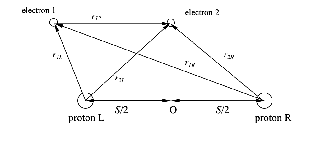
The system we will consider consists of two protons and two electrons. The protons are considered to be fixed (this is known as the Born-Oppenheimer approximation), and separated by a distance \(S\). For \(S \neq 0\), this represents a model of the \(H_2\) molecule, whereas for \(S=0\), we have a model of the Helium atom. The figure below shows the coordinates defined in the problem, with the position vectors \(\mathbf{r}_1\) and \(\mathbf{r}_2\) of electrons 1 and 2 are not shown for the sake of clarity.

The Schrödinger equation for the model can be separated into “nuclear” and “electronic” parts in the Born-Oppenheimer approximation.

The electronic part is given by:

\(\hat{H} \psi_e (r_1, r_2, S) = \left[ -\frac{\hbar^2}{2 m_e} (\nabla_1^2 + \nabla_2^2) + V(r_1, r_2) \right] \psi_e(r_1,r_2,S) = E_0 (S) \psi_e (r_1, r_2, S)\),

and the nuclear part:

\(\left[ \frac{\hbar^2}{2 m_p} \nabla_S^2 + \frac{e^2}{4\pi \epsilon_0 S} + E_0(S)\right] \psi_n (S) = \epsilon \psi_n(S)\),

where \(E_0(S)\) represents the electronic eigenvalue, \(\epsilon\) is the total energy of the system, \(m_{e,p}\) are the electron and proton masses respectively, and \(\psi_{e,n}\) are the electron and proton eigenfunctions, respectively, and \(V(r_1, r_2)\) is the electrostatic potential for the electrons.

Adopting “dimensionless atomic units”, i.e. setting \(a_0 = \frac{\hbar^2} {m_e e^2} \rightarrow 1\), where \(a_0\) is the Bohr radius, lengths are effectively given in Bohr radii. The resulting unit of energy is sometimes referred to as a “Hartree”, where 1 Hartree corresponds to \(\sim 27.192\) eV.

In these units, the electrostatic potential for the electrons, \(V(r_1, r_2)\), is given by:

\(V(r_1, r_2) = -\left[ \frac{1}{r_{1L}} + \frac{1}{r_{1R}} + \frac{1}{r_{2L}} + \frac{1}{r_{2R}} - \frac{1}{r_{12}}\right]\).

The potential governing the protons’ motion at a separation \(S (\neq 0)\), \(U(S)\) is the sum of the inter-proton electrostatic repulsion and the eigenvalue \(E_0(S)\) of the two-electron Schrödinger equation:

\(U(S) = \frac{1}{S} + E_0 (S)\).

Our goal here isa to obtain \(E_0(S)\), the electronic eigenvalue.

11.5.2. Variational Monte Carlo

Consider a Hamiltonian, \(\hat{H}\), for which we seek to estimate the ground state. The analytic variational method consists of constructing a “trial” wave function \(\psi_a\), which is parameterized by one or more variational parameters, \(a\). The expectation value of the energy is then calculated from:

\(\left< E(a) \right> = \frac{ \left< \psi_a | \hat{H} | \psi_a\right> } { \left< \psi_a| \psi_a\right> }\),

where the denominator is not necessary if the trial wave function is properly normalized.

The expectation value of the energy is then minimized with respect to the variational parameters, \(a\). The minimum value of \(\left< E(a) \right>\) yields an upper bound to the ground state energy of the system.

The Variational Monte Carlo (VMC) method seeks to minimize the energy numerically. In realistic systems, a many-body wave function assumes large values in small parts of the configuration space, and hence using homogeneously distributed random points to sample it is not sufficient. The algorithm of Metropolis et al. can be used to sample the required distribution, using an ensemble of random walkers moving through configuration space.

The trial wave function, denoted by \(\psi_T(\mathbf{x})\), is used to define the local energy:

\(E_L(\mathbf{x}) = \frac{ \hat{H} \psi_T } {\psi_T}\),

where \(\mathbf{x}\) is a multi-coordinate which represents the coordinates of all the particles in the system.

Using the above definition of the local energy, the expectation value of the energy can be written as:

\(\left< E\right> = \frac{ \int \mathrm{d} \mathbf{x} \psi^2_T(\mathbf{x}) E_L(\mathbf{x}) } { \int \mathrm{d} \mathbf{x} \psi^2_T(\mathbf{x}) }\).

The algorithm then consists of producing an initial random configuration of walkers that move around configuration space. The walker is moved within a distance \(d\) of about its initial position \(\mathbf{x}\), to a new position \(\mathbf{x}'\). The trial step is accepted or rejected, according to the usual Metropolis algorithm, with the ratio given by:

\(\rho = \frac{ \psi^2_T(\mathbf{x}') } { \psi^2_T(\mathbf{x})}\).

The expectation value of the energy is calculated by averaging the local energy over the random walk, taking into account the correct sampling interval, and excluding the thermalization steps at the start.

The size of the trial step can be chosen so that the acceptance ratio is equal to about \(0.5\) for each value of the variational parameter.

As a preparation to the full treatment of the \(He\) atom and \(H_2\) molecule, we investigate the Hydrogen atom in the following example. Note that a problem arises when attempting to calculate the auto-correlation function, because the trial wave function suggested by the problem is too close to the actual wave function. By examining the auto-correlation function, one notices that as \(a \rightarrow 1\) (i.e. as the trial function approaches the actual wave function), then \(C(k)\) becomes indeterminate, since the variance becomes zero at \(a=1\).

11.5.3. Example 11.2 Variational Monte Carlo for the Hydrogen Atom

Use the Variational Monte Carlo Method to calculate the ground state of the Hydrogen atom.

The Hamiltonian (energy) operator is:

\(\hat{H} = -\frac{1}{2} \nabla^2 - \frac{1}{r}\).

Use a trial wave function of the form:

\(\psi_a(r) = e^{-ar}\).

Note that for \(a=1\), the trial wave function becomes proportional to the exact ground state wave function.

The local energy for the H atom is:

\(E_L(r) = -\frac{1}{r} - \frac{1}{2} a \left( a - \frac{2}{r} \right)\).

Start with a set of \(N_w = 60\) walkers distributed at random in a cube of side \(d=20\).

Each walker should attempt trial steps by adding a random vector \(\Delta \mathbf{r}\) to the initial position \(\vec{r}\).

The trial step should be accepted or rejected according to the ratio:

\(\rho = \psi^2_a(\mathbf{r} + \Delta \mathbf{r}) / \psi^2_a (\mathbf{r})\).

The trial step can be varied from 0.5 to 1, adjusted to keep the acceptance ratio to \(\sim 0.5\) as we vary the parameter \(a\).

You may use a sampling interval of a length of \(\sim 25\). The minimum is expected to occur at \(a=1\), with an energy \(E=0.5=13.6\) eV, with zero variance!

11.5.4. VMC for the \(H_2\) Molecule and \(He\) Atom

The trial wave function suitable for the \(H_2\) problem is a special case of the Padé-Jastrow wave functions. It consists of a correlated product of molecular orbitals:

\(\Phi(\mathbf{r}_1, \mathbf{r}_2) = \phi(\mathbf{r}_1) \phi(\mathbf{r}_2) f(\mathbf{r}_{12})\),

where:

\(\phi(\mathbf{r}_i) = e^{-r_{iL}/c} + e^{-r_{iR}/c}\),

and

\(f(\mathbf{r}_{12}) = \exp \left[ \frac{r_{12}}{b(1 + a r_{12})} \right]\),

where \(a, b, c\) are variational parameters, and the coordinates are defined in the figure describing the model.

Certain conditions are imposed on these parameters, called “cusp” conditions, which cancel the divergences in the Coulomb potential as \(\mathbf{r}_{1L,R}, \mathbf{r}_{2L, R}, \mathbf{r}_{12} \rightarrow 0\).

To derive the cusp conditions, what needs to be considered for each vector separately is, e.g.:

\(\lim_{r_{1L} \rightarrow 0} \left[ - \frac{1}{2\phi(\mathbf{r}_1)} \nabla_1^2 \phi(\mathbf{r}_1) - \frac{1}{r_{1L}} \right] =\) finite terms.

After performing the differentiation for the Laplacian, the variational parameters \(b, c\) are chosen so as to cancel the negative divergence of the Coulomb potential. This procedure yields:

\(b=2\) and \(c = \frac{1}{1+ e^{-S/c}}\), where \(S\) is the inter-proton distance.

The second equation is transcendental and can be solved, e.g. via the Newton-Raphson method, each time the inter-proton separation is varied.

The remaining parameter, \(a\) can be varied in order to obtain the minimum variational energy.

What remains is to calculate the local energy for the system:

\(E_L(\mathbf{r}_1, \mathbf{r}_2) = \frac{\hat{H}\Phi(\mathbf{r}_1, \mathbf{r}_2)}{\Phi(\mathbf{r}_1, \mathbf{r}_2) } = \frac{1}{\Phi(\mathbf{r}_1, \mathbf{r}_2)} \left[ -\frac{\hbar^2}{2 m_e} (\nabla_1^2 + \nabla_2^2) + V(r_1, r_2) \right] \Phi(\mathbf{r}_1, \mathbf{r}_2)\).

The following identity can be employed:

\(\nabla_1^2 \left[ f(\mathbf{r}_{12}) \phi(\mathbf{r}_1) \right] = \phi(\mathbf{r}_1) \nabla^2_1 f(\mathbf{r}_{12}) + 2 \left[ \nabla_1 f(\mathbf{r}_12)\right] \cdot \left[ \nabla_1 \phi(\mathbf{r}_1)\right] + f(\mathbf{r}_{12}) \nabla^2_1 \phi(\mathbf{r}_1)\).

The distances to the “left” (L) and “right” (R) proton, and the inter-electron distance can be written as:

\(r_{iL} = \sqrt{ x_i^2 + y_i^2 + (z_1 + \frac{1}{2} S)^2}\),

\(r_{iR} = \sqrt{ x_i^2 + y_i^2 + (z_1 - \frac{1}{2} S)^2}\),

for \(i = 1,2\), and

\(r_{12} = \sqrt{ (x_1 - x_2)^2 + (y_1 - y_2)^2 + (z_1 - z_2)^2}\).

One finds that:

\(\nabla_i^2 \phi(\mathbf{r}_i) = -\frac{2}{c} \left[ \frac{e^{-r_{iL}/c}}{r_{iL}} + \frac{e^{-r_{iR}/c}}{r_{iR}} \right] + \frac{ \phi(\mathbf{r_i})}{c^2}\),

\(\nabla_i^2 f(\mathbf{r}_{12}) = f(\mathbf{r}_{12}) \left[ \frac{1}{b^2 ( 1 + a r_{12} )^4} + \frac{2}{b(1+a r_{12})^3 r_{12}} \right]\),

and

\(2 \left[ \nabla_1 f(\mathbf{r}_12)\right] \cdot \left[ \nabla_1 \phi(\mathbf{r}_1)\right] = \frac{2 (-1)^i f(\mathbf{r}_{12})}{bc(1 + ar_{12})^2 } \left[ \hat{\mathbf{r}}_{iL} \cdot \hat{\mathbf{r}}_{12} e^{-r_{iL}/c} + \hat{\mathbf{r}}_{iR} \cdot \hat{\mathbf{r}}_{12} e^{-r_{iR/c}}\right]\),

for \(i=1,2\), representing each electron.

Putting everything together, we obtain:

\(E_L(\mathbf{r}_1, \mathbf{r}_2) = V(\mathbf{r}_1, \mathbf{r}_2) + E_1 + E_2\), with:

\(E_i = -\frac{1}{2} \left[ \frac{1}{(1+ ar_{12})^3} + \frac{1}{c^2} + \frac{1}{4} \frac{1}{(1 + a r_{12})^4} - \frac{2}{c} \frac{ e^{r_{iL}/c}/r_{iL} + e^{r_{iR}/c}/r_{iR} } {e^{r_{iL}/c}+ e^{r_{iR}/c}} + \frac{(-1)^i}{c} \frac{1}{(1+a r_{12})^2} \frac{ e^{r_{iL}/c} \hat{\mathbf{r}}_{iL} \cdot \hat{\mathbf{r}}_{12} + e^{-r_{iR/c}}\hat{\mathbf{r}}_{iR} \cdot \hat{\mathbf{r}}_{12} }{e^{r_{iL}/c}+ e^{r_{iR}/c}} \right]\).

The Metropolis algorithm is applied in this case using a distribution of six-dimensional walkers, each representing the two electrons in the system. The minimum variational energy for the \(H_2\) molecule can be determined by varying the parameter \(a\) at each inter-proton separation \(S\). Note that the potential energy curve for the protons in this case needs to take into account the protons’ electrostatic repulsion.

To determine the upper bound for the ground state of the Helium atom, the inter-proton distance should be set to zero and the variational parameter should be varied.

11.5.5. Example 11.3 Variational Monte Carlo for the Helium Atom

Use the Variational Monte Carlo Method to calculate the ground state of the Helium atom (two protons in the nucleus).

Compare to the known value for the ground state energy of He: \(\simeq 79.005\) eV (https://www.nist.gov/pml/atomic-spectra-database)

You may use the local energy provided below:

def EnergyLocal(r, S, a):
    """Calculates the local energy for a 6-dimensional position vector r and interproton distance S and variational parameter a"""
    # get the components:
    r1x = r[0]
    r1y = r[1]
    r1z = r[2]
    r2x = r[3]
    r2y = r[4]
    r2z = r[5]
    
    # the vector connecting the electrons
    r12x = r1x - r2x
    r12y = r1y - r2y
    r12z = r1z - r2z

    # the unit vector connecting the electrons:
    r12 = np.sqrt(r12x**2 + r12y**2 + r12z**2)
    r12x = r12x / r12
    r12y = r12y / r12
    r12z = r12z / r12

    # get the unit vectors for proton L and R for electron 1
    r1L = np.sqrt(r1x**2 + r1y**2 + (r1z + (0.5 * S))**2)
    r1R = np.sqrt(r1x**2 + r1y**2 + (r1z - (0.5 * S))**2)
    r1Lx = r1x / r1L
    r1Ly = r1y / r1L
    r1Lz = (r1z + (0.5 * S)) / r1L
    r1Rx = r1x / r1R
    r1Ry = r1y / r1R
    r1Rz = (r1z - (0.5 * S)) / r1R

    # get the unit vectors for proton L and R for electron 2
    r2L = np.sqrt(r2x**2 + r2y**2 + (r2z + (0.5 * S))**2)
    r2R = np.sqrt(r2x**2 + r2y**2 + (r2z - (0.5 * S))**2)
    r2Lx = r2x / r2L
    r2Ly = r2y / r2L
    r2Lz = (r2z + (0.5 * S)) / r2L
    r2Rx = r2x / r2R;
    r2Ry = r2y / r2R;
    r2Rz = (r2z - (0.5 * S)) / r2R;
    # get the dot product between the unit vectors from protons L and R to electron 1 and the unit vector connecting
    # electrons 1 and 2:
    r1Lr12 = r1Lx * r12x + r1Ly * r12y + r1Lz * r12z;
    r1Rr12 = r1Rx * r12x + r1Ry * r12y + r1Rz * r12z;
    # get the dot product between the unit vectors from protons L and R to electron 2 and the unit vector connecting
    # electrons 1 and 2:
    r2Lr12 = r2Lx * r12x + r2Ly * r12y + r2Lz * r12z;
    r2Rr12 = r2Rx * r12x + r2Ry * r12y + r2Rz * r12z;

	#get c by solving the transcendetal equation
    c = NPsolve(S).x[0]
    
	#a is the variational param
    E1 = -0.5 * ( (( 1 + a * r12 )**(-3))/r12 + (1/c**2) + 0.25 * ( 1 + a * r12 )**(-4) - 
		(2 / c) * ( np.exp(-r1L / c)/r1L + np.exp(-r1R / c)/r1R) / ( np.exp(-r1L / c) + np.exp(-r1R / c) )
		- (1 / c) * (1+ a * r12)**(-2) * ( np.exp(-r1L / c) * r1Lr12 + np.exp(-r1R / c) * r1Rr12) / ( np.exp(-r1L / c) + np.exp(-r1R / c) ))

    
    E2 = -0.5 * ( (( 1 + a * r12 )**(-3))/r12 + (1/c**2) + 0.25 * ( 1 + a * r12 )**(-4) - 
		(2 / c) * ( np.exp(-r2L / c)/r2L + np.exp(-r2R / c)/r2R) / ( np.exp(-r2L / c) + np.exp(-r2R / c) )
     		+ (1 / c) * (1+ a * r12)**(-2) * ( np.exp(-r2L / c) * r2Lr12 + np.exp(-r2R / c) * r2Rr12) / ( np.exp(-r2L / c) + np.exp(-r2R / c) ))

    V = - 1/r1L - 1/r1R - 1/r2L - 1/r2R + 1/r12;

    # sum up and return
    #localE = V + E12 + E1 + E2
    localE = V + E1 + E2
    return localE

11.5.6. Example 11.4: Variational Monte Carlo for the Hydrogen Molecule

Use the Variational Monte Carlo Method to calculate the ground state of the Hydrogen molecule (\(H_2\)).